AI with rigor
Maximum Likelihood
Maximum likelihood estimation (MLE) finds the parameter values that maximize the likelihood function
$$ L(\theta) = P(\mathbf{x}|\theta) $$
given observed data $\mathbf{x} = {x_1, x_2, \ldots, x_n}$ and parameter vector $\theta$.
For independent observations, the likelihood becomes
$$ L(\theta) = \prod_{i=1}^n P(x_i|\theta) $$
and the MLE estimator is
In NLP, MLE is used to train language models by maximizing the probability of observed text sequences under the model parameters.
For a language model with parameters $\theta$, the MLE objective over a corpus of sequences ${w^{(1)}, w^{(2)}, \ldots, w^{(M)}}$ is
$$ \hat{\theta} = \arg\max_{\theta} \prod_{m=1}^M P(w^{(m)}|\theta) $$
Examples
Example 1: Language Model Training Given corpus: [“the cat”, “the dog”, “a cat”]
- Bigram model parameters: $P(\text{cat}|\text{the})$, $P(\text{dog}|\text{the})$, etc.
- MLE: $\hat{\theta} = \arg\max_{\theta} P(\text{the cat}|\theta) \times P(\text{the dog}|\theta) \times P(\text{a cat}|\theta)$
- Solution: $P(\text{cat}|\text{the}) = \frac{1}{2}$, $P(\text{dog}|\text{the}) = \frac{1}{2}$
Example 2: Neural Language Model For sequence “hello world” with vocabulary $V$:
- Model outputs: $P(w_t|w_{<t}, \theta)$ for each position $t$
- Likelihood: $L(\theta) = P(\text{hello}|\theta) \times P(\text{world}|\text{hello}, \theta)$
- MLE trains $\theta$ to maximize this probability
Example 3: Coin Flip Analogy Observed data: 7 heads, 3 tails in 10 flips
- Parameter: $p$ (probability of heads)
- Likelihood: $L(p) = \binom{10}{7} p^7 (1-p)^3$
- MLE solution: $\hat{p} = \frac{7}{10} = 0.7$
Maximum Log-Likelihood
Maximum log-likelihood estimation transforms the likelihood maximization problem into a more computationally tractable form by taking the logarithm: $$\hat{\theta} = \arg\max_{\theta} \log L(\theta) = \arg\max_{\theta} \log \prod_{i=1}^n P(x_i|\theta) = \arg\max_{\theta} \sum_{i=1}^n \log P(x_i|\theta)$$
The logarithm converts products to sums, preventing numerical underflow and making derivatives easier to compute. For language models, the negative log-likelihood (NLL) loss is commonly minimized: $$\mathcal{L}(\theta) = -\frac{1}{N} \sum_{i=1}^N \log P(w_i|w_{<i}, \theta)$$
where $N$ is the total number of tokens. This is equivalent to minimizing cross-entropy between the true distribution and model predictions. The log-likelihood objective is strictly concave for exponential family distributions, ensuring a unique global maximum.
Examples
Example 1: Numerical Stability Without log-likelihood:
- $P(w_1|\theta) = 0.1$, $P(w_2|\theta) = 0.05$, $P(w_3|\theta) = 0.02$
- Likelihood: $L(\theta) = 0.1 \times 0.05 \times 0.02 = 0.0001$ (underflow risk)
With log-likelihood:
- $\log L(\theta) = \log(0.1) + \log(0.05) + \log(0.02) = -2.3 + (-3.0) + (-3.9) = -9.2$
- Numerically stable and easier to optimize
Example 2: Cross-Entropy Loss True next word: “cat” (index 5 in vocabulary)
- Model output: $[0.1, 0.05, 0.15, 0.2, 0.1, 0.3, 0.1]$ (softmax probabilities)
- Log-likelihood: $\log P(\text{cat}) = \log(0.3) = -1.204$
- NLL loss: $-\log(0.3) = 1.204$ (lower is better)
Example 3: Training Objective For transformer language model on sequence “the cat sat”:
- Token probabilities: $P(\text{the}) = 0.8$, $P(\text{cat}|\text{the}) = 0.6$, $P(\text{sat}|\text{the cat}) = 0.4$
- Log-likelihood: $\log(0.8) + \log(0.6) + \log(0.4) = -0.223 + (-0.511) + (-0.916) = -1.65$
- Training maximizes this value (minimizes NLL = 1.65)
N-gram
An n-gram is a contiguous sequence of $n$ items from a given sequence of text or speech, where items are typically words, characters, or tokens. For a sequence $w_1, w_2, \ldots, w_m$, the set of all n-grams is ${w_i, w_{i+1}, \ldots, w_{i+n-1} : 1 \leq i \leq m-n+1}$.
In probabilistic language modeling, n-gram models estimate the probability of a word given the previous $n-1$ words using the Markov assumption:
$$ P(w_i | w_1, \ldots, w_{i-1}) \approx P(w_i | w_{i-n+1}, \ldots, w_{i-1}) $$
The maximum likelihood estimate for an n-gram probability is
$$ P(w_i | w_{i-n+1}, \ldots, w_{i-1}) = \frac{C(w_{i-n+1}, \ldots, w_i)}{C(w_{i-n+1}, \ldots, w_{i-1})} $$
where $C(\cdot)$ denotes the count function.
Examples
Example 1: Word N-grams from “The cat sat on the mat”
- Unigrams (1-grams): [“The”, “cat”, “sat”, “on”, “the”, “mat”]
- Bigrams (2-grams): [“The cat”, “cat sat”, “sat on”, “on the”, “the mat”]
- Trigrams (3-grams): [“The cat sat”, “cat sat on”, “sat on the”, “on the mat”]
- 4-grams: [“The cat sat on”, “cat sat on the”, “sat on the mat”]
Example 2: Character N-grams from “hello”
- Character bigrams: [“he”, “el”, “ll”, “lo”]
- Character trigrams: [“hel”, “ell”, “llo”]
- Useful for morphological analysis and handling out-of-vocabulary words
Example 3: Probability Calculation Given corpus with bigram counts:
- $C(\text{“the cat”}) = 15$, $C(\text{“the”}) = 100$
- $P(\text{cat} | \text{the}) = \frac{C(\text{“the cat”})}{C(\text{“the”})} = \frac{15}{100} = 0.15$
- For sentence probability: $P(\text{“the cat sat”}) = P(\text{the}) \times P(\text{cat} | \text{the}) \times P(\text{sat} | \text{cat})$
Dot Product
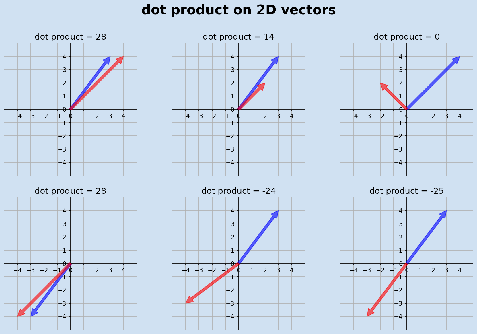
The dot product (or inner product) of two vectors $\mathbf{u}, \mathbf{v} \in \mathbb{R}^n$ is defined as
$$ \mathbf{u} \cdot \mathbf{v} = \sum_{i=1}^{n} u_i v_i = u_1 v_1 + u_2 v_2 + \cdots + u_n v_n $$.
Geometrically, it equals
$$ \mathbf{u} \cdot \mathbf{v} = |\mathbf{u}| |\mathbf{v}| \cos \theta $$
where $\theta$ is the angle between the vectors and $|\cdot|$ denotes the Euclidean norm. The dot product is commutative, distributive, and satisfies
$$ \mathbf{u} \cdot \mathbf{u} = |\mathbf{u}|^2 $$
In NLP, it serves as a fundamental similarity measure and is the core operation in attention mechanisms, where
$$ \text{score}(\mathbf{q}, \mathbf{k}) = \mathbf{q}^T \mathbf{k} $$
computes compatibility between query and key vectors.
Examples
Example 1: Word Embedding Similarity Given word embeddings:
- $\mathbf{v}_{\text{king}} = [0.2, 0.8, -0.1, 0.3]$
- $\mathbf{v}_{\text{queen}} = [0.1, 0.7, -0.2, 0.4]$
- Similarity = $\mathbf{u} \cdot \mathbf{v} = (0.2)(0.1) + (0.8)(0.7) + (-0.1)(-0.2) + (0.3)(0.4) = 0.72$
Example 2: Attention Score Computation In transformer attention:
- Query: $\mathbf{q} = [1, 2, 0]$
- Key: $\mathbf{k} = [2, 1, 3]$
- Raw attention score = $\mathbf{q} \cdot \mathbf{k} = (1)(2) + (2)(1) + (0)(3) = 4$
Example 3: Cosine Similarity Foundation For vectors $\mathbf{u} = [3, 4]$ and $\mathbf{v} = [1, 2]$:
- $\mathbf{u} \cdot \mathbf{v} = 3 \cdot 1 + 4 \cdot 2 = 11$
- $\cos \theta = \frac{\mathbf{u} \cdot \mathbf{v}}{|\mathbf{u}| |\mathbf{v}|} = \frac{11}{\sqrt{25} \sqrt{5}} = \frac{11}{5\sqrt{5}} \approx 0.98$
Cosine Similarity
Cosine similarity measures the cosine of the angle between two non-zero vectors $\mathbf{u}, \mathbf{v} \in \mathbb{R}^n$, defined as
$$ \cos(\theta) = \frac{\mathbf{u} \cdot \mathbf{v}}{|\mathbf{u}| |\mathbf{v}|} = \frac{\sum_{i=1}^{n} u_i v_i}{\sqrt{\sum_{i=1}^{n} u_i^2} \sqrt{\sum_{i=1}^{n} v_i^2}} $$
The similarity ranges from -1 (completely opposite) to 1 (identical direction), with 0 indicating orthogonality. Unlike Euclidean distance, cosine similarity is invariant to vector magnitude and focuses purely on orientation, making it ideal for high-dimensional sparse data like text embeddings. It is equivalent to the dot product of the L2-normalized vectors:
$$ \cos(\theta) = \frac{\mathbf{u}}{|\mathbf{u}|} \cdot \frac{\mathbf{v}}{|\mathbf{v}|} $$ .
Examples
Example 1: Document Similarity Given TF-IDF vectors:
- Document A: $\mathbf{d_A} = [3, 1, 0, 2]$
- Document B: $\mathbf{d_B} = [1, 2, 1, 0]$
- $\cos(\theta) = \frac{(3)(1) + (1)(2) + (0)(1) + (2)(0)}{\sqrt{9+1+0+4} \sqrt{1+4+1+0}} = \frac{5}{\sqrt{14} \sqrt{6}} = \frac{5}{\sqrt{84}} \approx 0.545$
Example 2: Word Embedding Comparison
- $\mathbf{v}_{happy} = [0.8, 0.3, -0.1]$
- $\mathbf{v}_{joyful} = [0.7, 0.4, -0.2]$
- $\cos(\theta) = \frac{(0.8)(0.7) + (0.3)(0.4) + (-0.1)(-0.2)}{\sqrt{0.64+0.09+0.01} \sqrt{0.49+0.16+0.04}} = \frac{0.56 + 0.12 + 0.02}{\sqrt{0.74} \sqrt{0.69}} \approx 0.98$
Example 3: Sentence Similarity in Practice Two sentences with BERT embeddings (768-dimensional):
- Sentence 1: “The cat is sleeping”
- Sentence 2: “A cat is napping”
- If cosine similarity = 0.85, this indicates high semantic similarity despite different words
Perplexity
Perplexity is the exponentiated cross-entropy of a probability distribution, formally defined as
$$ PP(W) = 2^{H(W)} $$
where $H(W)$ is the entropy of the word sequence $W$. For a language model with probability distribution $P$ over a test set of $N$ words, perplexity is computed as
$$PP = 2^{-\frac{1}{N} \sum_{i=1}^{N} \log_2 P(w_i | w_{<i})}$$
Equivalently, it can be expressed as the geometric mean of the reciprocal probabilities:
$$PP = \sqrt[N]{\prod_{i=1}^{N} \frac{1}{P(w_i | w_{<i})}}$$
Lower perplexity indicates better predictive performance, with a perfect model achieving perplexity of 1.
Examples
Example 1: Simple Bigram Model Given the sentence “the cat sat” and a bigram model:
- $P(\text{cat} | \text{the}) = 0.3$
- $P(\text{sat} | \text{cat}) = 0.2$
- Perplexity = $\sqrt{\frac{1}{0.3} \times \frac{1}{0.2}} = \sqrt{16.67} \approx 4.08$
Example 2: Comparative Analysis
- Model A: Perplexity = 50 on test set
- Model B: Perplexity = 25 on test set
- Model B is better, as it’s less “perplexed” by the test data
Example 3: Practical Context State-of-the-art language models typically achieve:
- Penn Treebank: ~50-60 perplexity
- WikiText-2: ~30-40 perplexity
- Large transformer models can achieve much lower perplexity on these benchmarks
Transformer Model
The original Transformer is a sequence-to-sequence model based entirely on attention mechanisms, eschewing recurrence and convolution. The model consists of an encoder-decoder architecture where the encoder maps an input sequence $(x_1, \ldots, x_n)$ to a sequence of continuous representations $\mathbf{z} = (z_1, \ldots, z_n)$, and the decoder generates an output sequence $(y_1, \ldots, y_m)$ one element at a time given $\mathbf{z}$ and previously generated symbols. Each encoder and decoder layer contains multi-head self-attention and position-wise feed-forward networks with residual connections and layer normalization. The model’s core innovation is the scaled dot-product attention mechanism:
$$ \text{Attention}(\mathbf{Q}, \mathbf{K}, \mathbf{V}) = \text{softmax}\left(\frac{\mathbf{Q}\mathbf{K}^T}{\sqrt{d_k}}\right)\mathbf{V} $$
Examples
Example 1: Translation Task
- Input: “Hello world” → Encoder processes with self-attention
- Encoder output: Contextual representations $[\mathbf{z}_1, \mathbf{z}_2]$
- Decoder generates: “Bonjour” (attending to encoder states), then “monde” (attending to encoder + “Bonjour”)
Example 2: Architecture Dimensions
- Model dimension $d_{model} = 512$
- 6 encoder layers, 6 decoder layers
- 8 attention heads with $d_k = d_v = 64$
- Feed-forward dimension $d_{ff} = 2048$
Example 3: Attention Pattern In “The cat sat on the mat”:
- Word “sat” attends strongly to “cat” (subject-verb relation)
- Word “mat” attends to “the” (determiner-noun relation)
- Self-attention captures these dependencies without recurrence
Self-Attention
Self-attention is an attention mechanism where queries, keys, and values are all derived from the same input sequence $\mathbf{X} \in \mathbb{R}^{n \times d}$, computed as
$\mathbf{Q} = \mathbf{X}\mathbf{W}^Q$, $\mathbf{K} = \mathbf{X}\mathbf{W}^K$, $\mathbf{V} = \mathbf{X}\mathbf{W}^V$
where $\mathbf{W}^Q, \mathbf{W}^K, \mathbf{W}^V \in \mathbb{R}^{d \times d_k}$ are learned parameter matrices.
The attention output is $Z = \text{softmax}\left(\frac{QK^T}{\sqrt{d_k}}\right)V$, where each output position $z_i$ is a weighted combination of all input positions. The attention weights
$$ \alpha_{ij} = \frac{\exp(q_i^T k_j / \sqrt{d_k})}{\sum_{l=1}^n \exp(q_i^T k_l / \sqrt{d_k})} $$
represent how much position $i$ attends to position $j$.
This mechanism allows each position to attend to all positions in the input sequence, capturing long-range dependencies in a single layer.
Examples
Example 1: Pronoun Resolution Input: “The cat ate its food”
- When processing “its”, self-attention assigns high weight to “cat”
- Attention weights: $\alpha_{\text{its},\text{cat}} = 0.8$, $\alpha_{\text{its},\text{food}} = 0.15$
- Output representation of “its” incorporates information from “cat”
Example 2: Computation for Short Sequence Input embeddings: $\mathbf{X} = [\mathbf{x}_1, \mathbf{x}_2, \mathbf{x}_3]^T$
- $\mathbf{Q} = \mathbf{X}\mathbf{W}^Q$, $\mathbf{K} = \mathbf{X}\mathbf{W}^K$, $\mathbf{V} = \mathbf{X}\mathbf{W}^V$
- Attention matrix: $\mathbf{A} = \text{softmax}\left(\frac{\mathbf{Q}\mathbf{K}^T}{\sqrt{d_k}}\right) \in \mathbb{R}^{3 \times 3}$
- Each row sums to 1, showing how each position attends to all positions
Example 3: Syntactic Dependencies In “The quick brown fox jumps”:
- “fox” (position 4) attends to “The” (0.1), “quick” (0.3), “brown” (0.6)
- Self-attention learns that adjectives modify the noun without explicit syntax
Multi-Head Attention
Multi-head attention performs $h$ different attention computations in parallel, each with different learned projections, formally defined as
$$ \text{MultiHead}(\mathbf{Q}, \mathbf{K}, \mathbf{V}) = \text{Concat}(\text{head}_1, \ldots, \text{head}_h)\mathbf{W}^O $$
where
$$\text{head}_i = \text{Attention}(\mathbf{Q}\mathbf{W}_i^Q, \mathbf{K}\mathbf{W}_i^K, \mathbf{V}\mathbf{W}_i^V)$$
Each head has parameter matrices $$W_i^Q, W_i^K, W_i^V \in \mathbb{R}^{d_{model} \times d_k}$$ where typically $$d_k = d_v = d_{model}/h$$ and $$W^O \in \mathbb{R}^{hd_v \times d_{model}}$$ is the output projection.
This allows the model to jointly attend to information from different representation subspaces at different positions, with each head potentially capturing different types of relationships (syntactic, semantic, positional). The computational complexity remains $O(n^2 d)$ where $n$ is sequence length and $d$ is model dimension.
Examples
Example 1: Different Head Specializations In “The cat sat on the mat”:
- Head 1: Focuses on subject-verb relationships (cat ↔ sat)
- Head 2: Captures determiner-noun pairs (The ↔ cat, the ↔ mat)
- Head 3: Handles prepositional phrases (sat ↔ on, on ↔ mat)
- Head 4: Long-range dependencies (cat ↔ mat)
Example 2: Dimensional Example For $d_{model} = 512$ and $h = 8$ heads:
- Each head: $d_k = d_v = 512/8 = 64$
- Head computations: $\mathbf{Q}_i, \mathbf{K}_i, \mathbf{V}_i \in \mathbb{R}^{n \times 64}$
- Concatenated output: $\mathbb{R}^{n \times 512}$ before final projection
- Total parameters per layer: $4 \times 512 \times 512 = 1,048,576$
Example 3: Attention Pattern Analysis Given sentence “She gave him the book”:
- Head 1 attention weights: she→gave (0.9), him→gave (0.8)
- Head 2 attention weights: book→the (0.7), book→gave (0.6)
- Combined representation captures both grammatical and semantic relationships
Add & Norm
Add & Norm refers to the residual connection followed by layer normalization applied around each sub-layer in the Transformer, formally expressed as $$\text{LayerNorm}(\mathbf{x} + \text{Sublayer}(\mathbf{x}))$$
where $\text{Sublayer}(\mathbf{x})$ is the output of the sub-layer (attention or feed-forward). Layer normalization is defined as $$\text{LayerNorm}(\mathbf{x}) = \frac{\mathbf{x} - \boldsymbol{\mu}}{\boldsymbol{\sigma}} \odot \boldsymbol{\gamma} + \boldsymbol{\beta}$$ where $$\boldsymbol{\mu} = \frac{1}{d}\sum_{i=1}^d x_i$$
$$\boldsymbol{\sigma} = \sqrt{\frac{1}{d}\sum_{i=1}^d (x_i - \mu)^2}$$
and $\boldsymbol{\gamma}, \boldsymbol{\beta} \in \mathbb{R}^d$ are learnable parameters. The residual connection enables gradient flow through deep networks by providing a direct path, while layer normalization stabilizes training by normalizing activations across the feature dimension for each sample independently.
Examples
Example 1: Residual Connection Impact Input: $\mathbf{x} = [1.0, 2.0, 0.5]$
- Multi-head attention output: $\text{MHA}(\mathbf{x}) = [0.2, -0.3, 0.8]$
- After residual: $\mathbf{x} + \text{MHA}(\mathbf{x}) = [1.2, 1.7, 1.3]$
- Preserves original information while adding learned representations
Example 2: Layer Normalization Computation For vector $\mathbf{h} = [2.0, 4.0, 1.0, 3.0]$:
- Mean: $\mu = \frac{2+4+1+3}{4} = 2.5$
- Variance: $\sigma^2 = \frac{(2-2.5)^2+(4-2.5)^2+(1-2.5)^2+(3-2.5)^2}{4} = 1.25$
- Normalized: $\frac{[2,4,1,3] - 2.5}{\sqrt{1.25}} = [-0.45, 1.34, -1.34, 0.45]$
Example 3: Training Stability Without Add & Norm:
- Gradients can vanish in deep networks (50+ layers)
- Activation distributions shift during training With Add & Norm:
- Enables training of very deep Transformers (100+ layers)
- Stable gradients and faster convergence
Feed Forward
The position-wise feed-forward network (FFN) in Transformers is a two-layer fully connected network with ReLU activation, applied identically to each position:
$$ \text{FFN}(x) = \max(0, xW_1 + b_1)W_2 + b_2 $$
where $$W_1 \in \mathbb{R}^{d_{model} \times d_{ff}}$$
$$W_2 \in \mathbb{R}^{d_{ff} \times d_{model}}$$
$$b_1 \in \mathbb{R}^{d_{ff}}$$
$$b_2 \in \mathbb{R}^{d_{model}}$$ are learnable parameters.
The inner dimension $d_{ff}$ is typically $4 \times d_{model}$, creating a bottleneck architecture that first expands then compresses the representation. This component processes each position independently, providing the model with non-linear transformation capabilities and increasing representational capacity. The FFN accounts for approximately two-thirds of the model’s parameters.
Example 1: Dimensional Transformation For $d_{model} = 512$ and $d_{ff} = 2048$:
- Input: $\mathbf{x} \in \mathbb{R}^{512}$
- After first layer: $\mathbf{h} = \text{ReLU}(\mathbf{x}\mathbf{W}_1 + \mathbf{b}_1) \in \mathbb{R}^{2048}$
- After second layer: $\text{FFN}(\mathbf{x}) = \mathbf{h}\mathbf{W}_2 + \mathbf{b}_2 \in \mathbb{R}^{512}$
- Parameters: $512 \times 2048 + 2048 \times 512 = 2,097,152$ weights
Example 2: Position-wise Processing Input sequence: $\mathbf{X} = [\mathbf{x}_1, \mathbf{x}_2, \mathbf{x}_3] \in \mathbb{R}^{3 \times 512}$
- Each position processed independently: $\text{FFN}(\mathbf{x}_i)$ for $i = 1,2,3$
- Same parameters $\mathbf{W}_1, \mathbf{W}_2$ applied to all positions
- Output: $[\text{FFN}(\mathbf{x}_1), \text{FFN}(\mathbf{x}_2), \text{FFN}(\mathbf{x}_3)]$
Example 3: Non-linear Transformation Input: $\mathbf{x} = [0.5, -0.3, 0.8]$
- First layer: $\mathbf{h} = \text{ReLU}([\mathbf{x}\mathbf{W}_1 + \mathbf{b}_1]) = [2.1, 0.0, 1.4, 0.7]$
- Second layer: $\text{FFN}(\mathbf{x}) = \mathbf{h}\mathbf{W}_2 + \mathbf{b}_2 = [0.9, -0.1, 1.2]$
- Provides non-linear processing between attention layers
Softmax
The softmax function transforms a vector of real numbers into a probability distribution, defined as
$$\text{softmax}(z_i) =\frac{\exp(z_i)}{\sum_{j=1}^K \exp(z_j)}$$
$$\text{for i = 1, 2, …, K}$$ where $$z = [z_1, z_2, …, z_K]^T$$
The output satisfies $$\sum_{i=1}^K \text{softmax}(z)_i = 1$$ and $$\text{softmax}(z)_i > 0$$ for all $i$, making it a valid probability distribution.
In Transformers, softmax is applied to attention scores $\frac{QK^T}{\sqrt{d_k}}$ to obtain attention weights, and to final layer outputs for classification tasks. The function is temperature-controlled: $\text{softmax}(z/\tau)$ where $\tau > 0$ controls the sharpness of the distribution.
Examples
Example 1: Attention Weight Computation Raw attention scores: $\mathbf{s} = [2.0, 1.0, 3.0]$
- Exponentials: $[\exp(2.0), \exp(1.0), \exp(3.0)] = [7.39, 2.72, 20.09]$
- Sum: $7.39 + 2.72 + 20.09 = 30.20$
- Softmax: $[7.39/30.20, 2.72/30.20, 20.09/30.20] = [0.245, 0.090, 0.665]$
- Highest score gets most attention weight
Example 2: Temperature Effect Logits: $\mathbf{z} = [1.0, 2.0, 3.0]$
- $\tau = 1.0$: $\text{softmax}(\mathbf{z}) = [0.090, 0.244, 0.666]$
- $\tau = 0.5$: $\text{softmax}(\mathbf{z}/0.5) = [0.018, 0.118, 0.864]$ (sharper)
- $\tau = 2.0$: $\text{softmax}(\mathbf{z}/2.0) = [0.186, 0.307, 0.507]$ (smoother)
Example 3: Numerical Stability Unstable: $\mathbf{z} = [1000, 1001, 1002]$ causes overflow
- Stable computation: $\mathbf{z}’ = \mathbf{z} - \max(\mathbf{z}) = [0, 1, 2]$
- $\text{softmax}(\mathbf{z}’) = [0.090, 0.244, 0.666]$
- Subtracting maximum prevents numerical overflow
Positional Embeddings
Positional embeddings provide sequence position information to the Transformer, which lacks inherent position awareness due to the permutation-invariant nature of attention. The original Transformer uses sinusoidal positional encoding: $$PE_{(pos,2i)} = \sin(pos/10000^{2i/d_{model}})$$ and $$PE_{(pos,2i+1)} = \cos(pos/10000^{2i/d_{model}})$$ where $pos$ is the position and $i$ is the dimension index.
These encodings are added to input embeddings:
Examples
Example 1: Sinusoidal Encoding Values For $d_{model} = 4$ and positions 0, 1, 2:
- Position 0: $[0, 1, 0, 1]$ (sin(0), cos(0), sin(0), cos(0))
- Position 1: $[0.841, 0.540, 0.010, 0.9999]$
- Position 2: $[0.909, -0.416, 0.020, 0.9998]$
- Each position has unique encoding pattern
Example 2: Frequency Pattern For dimension $i = 0, 1, 2, 3$ in $d_{model} = 512$:
- $i = 0$: frequency $= 1/10000^{0/512} = 1.0$ (high frequency)
- $i = 256$: frequency $= 1/10000^{256/512} = 0.1$ (medium frequency)
- $i = 511$: frequency $= 1/10000^{511/512} \approx 0.0001$ (low frequency)
- Different dimensions capture different temporal scales
Example 3: Learned vs Fixed Embeddings Input: “The cat sat” (positions 0, 1, 2)
- Fixed sinusoidal: Same encoding for all models and training runs
- Learned embeddings often perform slightly better but less interpretable
Queries, Keys, Values
Queries (Q), Keys (K), and Values (V) are the fundamental components of attention mechanisms, derived from input representations through learned linear transformations:
$$\mathbf{Q} = \mathbf{X}\mathbf{W}^Q$$
$$\mathbf{K} = \mathbf{X}\mathbf{W}^K$$
$$\mathbf{V} = \mathbf{X}\mathbf{W}^V$$
where $$\mathbf{X} \in \mathbb{R}^{n \times d}$$ is the input and $$\mathbf{W}^Q, \mathbf{W}^K, \mathbf{W}^V \in \mathbb{R}^{d \times d_k}$$ are parameter matrices. The attention mechanism computes similarity between queries and keys to determine attention weights:
This design enables flexible attention patterns where each query can attend to any key-value pair based on learned similarity.
Examples
Example 1: Information Retrieval Analogy Query: “Find papers about neural networks”
- Keys: Paper titles/abstracts in database
- Values: Full paper content or metadata
- Attention: Compute similarity between query and all keys
- Output: Weighted combination of values based on relevance
Example 2: Self-Attention Computation Input: $\mathbf{X} = [\mathbf{x}_1, \mathbf{x}_2, \mathbf{x}_3]$ representing “cat sat mat”
- $\mathbf{Q} = \mathbf{K} = \mathbf{V} = \mathbf{X}\mathbf{W}$ (same source)
- Query “sat” ($\mathbf{q}_2$) computes similarity with all keys
- High similarity with “cat” key → high attention weight
- Output combines values weighted by attention
Example 3: Cross-Attention in Decoder Encoder outputs: $\mathbf{Z} = [\mathbf{z}_1, \mathbf{z}_2, \mathbf{z}_3]$ (“Hello world”)
- Keys and Values: $\mathbf{K} = \mathbf{V} = \mathbf{Z}\mathbf{W}$ (from encoder)
- Query: $\mathbf{Q} = \mathbf{Y}\mathbf{W}^Q$ (from decoder, e.g., “Bonjour”)
- Decoder attends to relevant encoder positions for translation
Residual Connection
A residual connection, also known as a skip connection, adds the input of a layer directly to its output, formally expressed as $$\mathbf{y} = \mathbf{x} + F(\mathbf{x})$$ where $\mathbf{x}$ is the input, $F(\mathbf{x})$ is the layer’s transformation, and $\mathbf{y}$ is the final output.
In Transformers, residual connections are applied around both multi-head attention and feed-forward sublayers:
and
Examples
Example 1: Gradient Flow Deep network without residuals:
- Gradient:
With residuals:
- Gradient: $$\frac{\partial \mathbf{x}_{i+1}}{\partial \mathbf{x}_i} = \mathbf{I} + \frac{\partial F(\mathbf{x}_i)}{\partial \mathbf{x}_i}$$
- Identity matrix ensures gradient flow even if $F$ contributes little
Example 2: Concrete Computation Input: $\mathbf{x} = [1.0, 2.0, 0.5]$
- Attention output: $\text{Attention}(\mathbf{x}) = [0.3, -0.1, 0.8]$
- With residual: $\mathbf{y} = [1.0, 2.0, 0.5] + [0.3, -0.1, 0.8] = [1.3, 1.9, 1.3]$
- Preserves original information while adding learned features
Example 3: Training Dynamics Early training: $F(\mathbf{x}) \approx \mathbf{0}$ (random initialization)
- Output: $\mathbf{y} = \mathbf{x} + \mathbf{0} = \mathbf{x}$ (identity function)
- Model can learn incrementally from identity baseline Later training: $F(\mathbf{x})$ becomes more meaningful
- Model learns to add useful transformations to the residual stream
Encoder-Decoder
The encoder-decoder architecture consists of two main components: an encoder that maps input sequence $\mathbf{x} = (x_1, \ldots, x_n)$ to continuous representations $\mathbf{z} = (z_1, \ldots, z_n)$, and a decoder that generates output sequence $\mathbf{y} = (y_1, \ldots, y_m)$ conditioned on $\mathbf{z}$.
The encoder uses self-attention layers: $$\mathbf{z}^{(l)} = \text{EncoderLayer}^{(l)}(\mathbf{z}^{(l-1)})$$ for $l = 1, \ldots, L$, while the decoder combines masked self-attention and cross-attention: $$\mathbf{h}^{(l)} = \text{DecoderLayer}^{(l)}(\mathbf{h}^{(l-1)}, \mathbf{z}^{(L)})$$. The decoder generates outputs autoregressively: $$P(\mathbf{y} | \mathbf{x}) = \prod_{t=1}^m P(y_t | y_{<t}, \mathbf{z})$$ where $y_{<t}$ represents previously generated tokens. Cross-attention in the decoder allows each output position to attend to all encoder positions, enabling flexible alignment between input and output sequences.
Examples
Example 1: Machine Translation Input: “Je suis étudiant” (encoder processes entire sequence)
- Encoder: Generates contextual representations for each French word
- Decoder step 1: Generates “I” (attending to “Je”)
- Decoder step 2: Generates “am” (attending to “suis”, aware of “I”)
- Decoder step 3: Generates “student” (attending to “étudiant”, aware of “I am”)
Example 2: Attention Patterns Encoder self-attention: Each French word attends to all French words
- “étudiant” attends to “Je” (0.3), “suis” (0.2), “étudiant” (0.5) Decoder cross-attention: Each English word attends to all French words
- “student” attends to “Je” (0.1), “suis” (0.1), “étudiant” (0.8) Decoder self-attention: Each English word attends to previous English words
- “student” attends to “I” (0.4), “am” (0.6), masked from future
Example 3: Computational Flow Encoder: $\mathbf{X} \rightarrow \mathbf{Z}$ (parallel processing)
- All positions processed simultaneously
- Bidirectional context (each position sees all others) Decoder: $\mathbf{Z}, \mathbf{Y}_{<t} \rightarrow y_t$ (sequential generation)
- Autoregressive: must generate tokens one by one
- Causal masking: position $t$ only sees positions $< t$
Scaled Dot-Product Attention
Scaled dot-product attention is the core attention mechanism in Transformers, defined as $$\text{Attention}(\mathbf{Q}, \mathbf{K}, \mathbf{V}) = \text{softmax}\left(\frac{\mathbf{Q}\mathbf{K}^T}{\sqrt{d_k}}\right)\mathbf{V}$$ where $$\mathbf{Q} \in \mathbb{R}^{n \times d_k}$$ $$\mathbf{K} \in \mathbb{R}^{m \times d_k}$$ and $$\mathbf{V} \in \mathbb{R}^{m \times d_v}$$ are query, key, and value matrices respectively.
The scaling factor $\sqrt{d_k}$ prevents the dot products from becoming too large, which would push the softmax function into regions with extremely small gradients. The attention weights $$\mathbf{A} = \text{softmax}\left(\frac{\mathbf{Q}\mathbf{K}^T}{\sqrt{d_k}}\right) \in \mathbb{R}^{n \times m}$$ represent how much each query position attends to each key position. The computational complexity is $O(n^2 d_k + nmd_v)$ where $n$ is the sequence length.
Examples
Example 1: Scaling Factor Importance Without scaling ($d_k = 64$):
- Dot product: $\mathbf{q}^T\mathbf{k} = 8.0$ (typical magnitude)
- Softmax input: $[8.0, 2.0, 1.0]$
- Softmax output: $[0.997, 0.002, 0.001]$ (too sharp)
With scaling:
- Scaled dot product: $\mathbf{q}^T\mathbf{k} / \sqrt{64} = 1.0$
- Softmax input: $[1.0, 0.25, 0.125]$
- Softmax output: $[0.576, 0.261, 0.163]$ (balanced)
Example 2: Step-by-Step Computation Given $\mathbf{Q} = \begin{bmatrix} 1 & 2 \ 0 & 1 \end{bmatrix}$, $\mathbf{K} = \begin{bmatrix} 2 & 1 \ 1 & 3 \end{bmatrix}$, $\mathbf{V} = \begin{bmatrix} 0.5 & 1.0 \ 1.5 & 0.5 \end{bmatrix}$, $d_k = 2$:
- $\mathbf{Q}\mathbf{K}^T = \begin{bmatrix} 4 & 7 \ 1 & 3 \end{bmatrix}$
- Scaled: $\frac{\mathbf{Q}\mathbf{K}^T}{\sqrt{2}} = \begin{bmatrix} 2.83 & 4.95 \ 0.71 & 2.12 \end{bmatrix}$
- Softmax: $\mathbf{A} = \begin{bmatrix} 0.23 & 0.77 \ 0.24 & 0.76 \end{bmatrix}$
Sequence-to-Sequence (Seq2Seq)
Sequence-to-sequence models map input sequences $$X = (x_1, x_2, \ldots, x_T)$$
to output sequences $$Y = (y_1, y_2, \ldots, y_{T’})$$ of potentially different lengths, using an encoder-decoder framework with the conditional probability $$P(Y|X) = \prod_{t=1}^{T’} P(y_t | y_{<t}, X)$$
The encoder computes a fixed-size context vector $$c = f(x_1, x_2, \ldots, x_T)$$ that summarizes the input sequence, while the decoder generates outputs autoregressively: $$P(y_t | y_{<t}, X) = g(y_{t-1}, s_t, c)$$ where $s_t$ is the decoder hidden state. In RNN-based seq2seq, the encoder final state initializes the decoder: $$s_0 = h_T^{enc}$$ and $$s_t = f_{dec}(y_{t-1}, s_{t-1}, c)$$
Modern implementations use attention mechanisms to replace the fixed context vector with dynamic context: $$c_t = \sum_{i=1}^T \alpha_{ti} h_i^{enc}$$ where attention weights $$\alpha_{ti}$$ focus on relevant encoder positions.
Examples
Example 1: Machine Translation Input (English): “I love cats” → $X = [x_1, x_2, x_3]$
- Encoder: Processes entire English sentence → context vector $c$
- Decoder step 1: $P(y_1|c) =$ “J’” (French for “I”)
- Decoder step 2: $P(y_2|y_1, c) =$ “aime” (given “J’”)
- Decoder step 3: $P(y_3|y_1, y_2, c) =$ “les”
- Output: “J’aime les chats”
Example 2: Text Summarization Input: Long news article (500 tokens)
- Encoder: $h_1, h_2, \ldots, h_{500}$ (bidirectional LSTM states)
- Context: $c = \text{mean}(h_1, \ldots, h_{500})$ or $c = h_{500}^{forward} + h_1^{backward}$
- Decoder: Generates summary tokens one by one
- Output: Short summary (50 tokens)
Example 3: Attention-Based Seq2Seq Input: “The quick brown fox”
- Encoder states: $[h_1^{enc}, h_2^{enc}, h_3^{enc}, h_4^{enc}]$
- Decoder at timestep $t$: Computes attention over all encoder states
- $\alpha_{t1} = 0.1, \alpha_{t2} = 0.6, \alpha_{t3} = 0.2, \alpha_{t4} = 0.1$
- Dynamic context: $c_t = 0.1 \cdot h_1 + 0.6 \cdot h_2 + 0.2 \cdot h_3 + 0.1 \cdot h_4$
- Allows decoder to focus on relevant input parts for each output