The Du Compiler:

This is the naive/brute-force implementation of the Mandelbrot Set plotting. I just followed the algorithm.

# Plotting the Mandelbrot Set 

# length of sequence for real and imaginary parts of complex numbers
length <- 1000

# sequences for real and imaginary parts
real = seq(-1.8,0.6, len=length)
imaginary = seq(-1.2,1.2, len=length)


result <- matrix(nrow = length, ncol = length)

for (i in 1:length)
{
  for (j in 1:length)
  {
    result[i,j]=inmandelbrotset(complex(real = real[i], imaginary = imaginary[j]))       
  }
}

image(result, axes=FALSE)



# function that checks if a point E mandelbrot set
inmandelbrotset <- function(c)
{
  dwell.limit <- 2048
  z <- 0  
  for (i in 1:dwell.limit)
  { 
    z <- z ** 2 + c
    if (Mod(z) > 2)
    {
      return(FALSE)
    }
  }  
  return(TRUE)
}

Adding colors: We now have a Boolean matrix that records if a point is in the Mandelbrot Set. Since the matrix can only have two values : true or false, thus far, we have only been able to plot read and white images. The next step is to add colors such that we get more information on when a particular point escapes the radius of 2. Again, this is the naive/brute force way of doing it.

# Mandelbrot Plotting with colors 
length <- 1000
real = seq(-2.0,2.0, len=length)
imaginary = seq(-2.0,2.0, len=length)
result <- matrix(nrow = length, ncol = length)
dwell.limit <- 512

for (i in 1:length)
{
  for (j in 1:length)
  {  
    z <- 0
    c <-complex(real = real[i], imaginary = imaginary[j])
    for (k in 1:dwell.limit)
    { 
      
      z <- z ** 2 + c
      if (Mod(z) > 2)
      {      
        result[i,j]=k
        break
      }
    }     
    
  }
}
set.seed(2)
image(result,breaks=0:dwell.limit
      ,col=c(1,sample(terrain.colors
                      (dwell.limit-1,alpha = .8))),asp=1,ax=F)

and, just for the heck of it..

ASCII Mandelbrot Set using R (naive)

s <- seq(-1.7,1.2, by =.1)
a <- ""
for (i in 1:length(s))
{  
  for (j in 1:length(s))
  {
   a<-cat(a,inmandelbrotset(complex(r = s[j], i = s[i])))     
  }  
  a <- cat(a,"\n")
}

Achieved by returning a " " or “#” instead of FALSE or TRUE from function “inmandelbrotset”. A better algorithm Utilizing R’s easy to use lists in implementation:

# more efficient algorithm to plot the Mandelbrot set 

sequence <- seq(-2,2,len=1000)
dwell.limit <- 200

# matrix of points to be iterated 
complex.matrix <- t((sapply(sequence,function(x)x+1i*sequence)))
in.mandelbrot.index <- 1:length(complex.matrix)
iter=z=array(0,dim(complex.matrix)) 
           
for(i in 1:dwell.limit){ 
  # complex quadratic polynomial function for all points
  z[in.mandelbrot.index]=complex.matrix[in.mandelbrot.index]+z[in.mandelbrot.index]^2 
  # boolean matrix
  result=Mod(z[in.mandelbrot.index])<=2  
  # if result is false, store the iteration 
  iter[in.mandelbrot.index[!result]]=i
  # save all the index where points are still in the mandelbrot
  in.mandelbrot.index=in.mandelbrot.index[result]
}
set.seed(19)
image(iter,main=paste("Iterations: ", i, sep=" "), breaks=0:dwell.limit
      ,col=c(1,sample(rainbow
                      (dwell.limit-1,alpha = .8))),ax=F, asp=1)

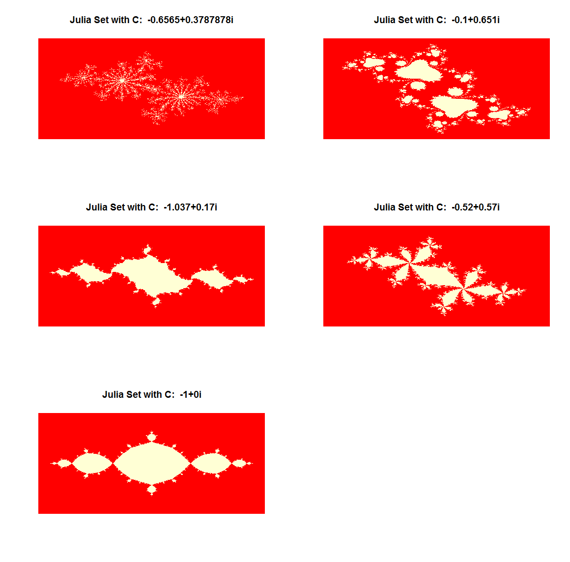
Plotting the Julia set A little modification to the code above (red and white Mandelbrot) produces Julia Sets. The idea here is to set a constant C and send Z to the function instead of C.

c <- complex(real=-0.1,imaginary=0.651) 
label <- toString(c)
injulia <- function(z)
{
  dwell.limit <- 128
  
  for (i in 1:dwell.limit)
  { 
    z <- z ** 2 + c
    if (Mod(z) > 2)
    {
      return(FALSE)
    }
  }  
  return(TRUE)
}

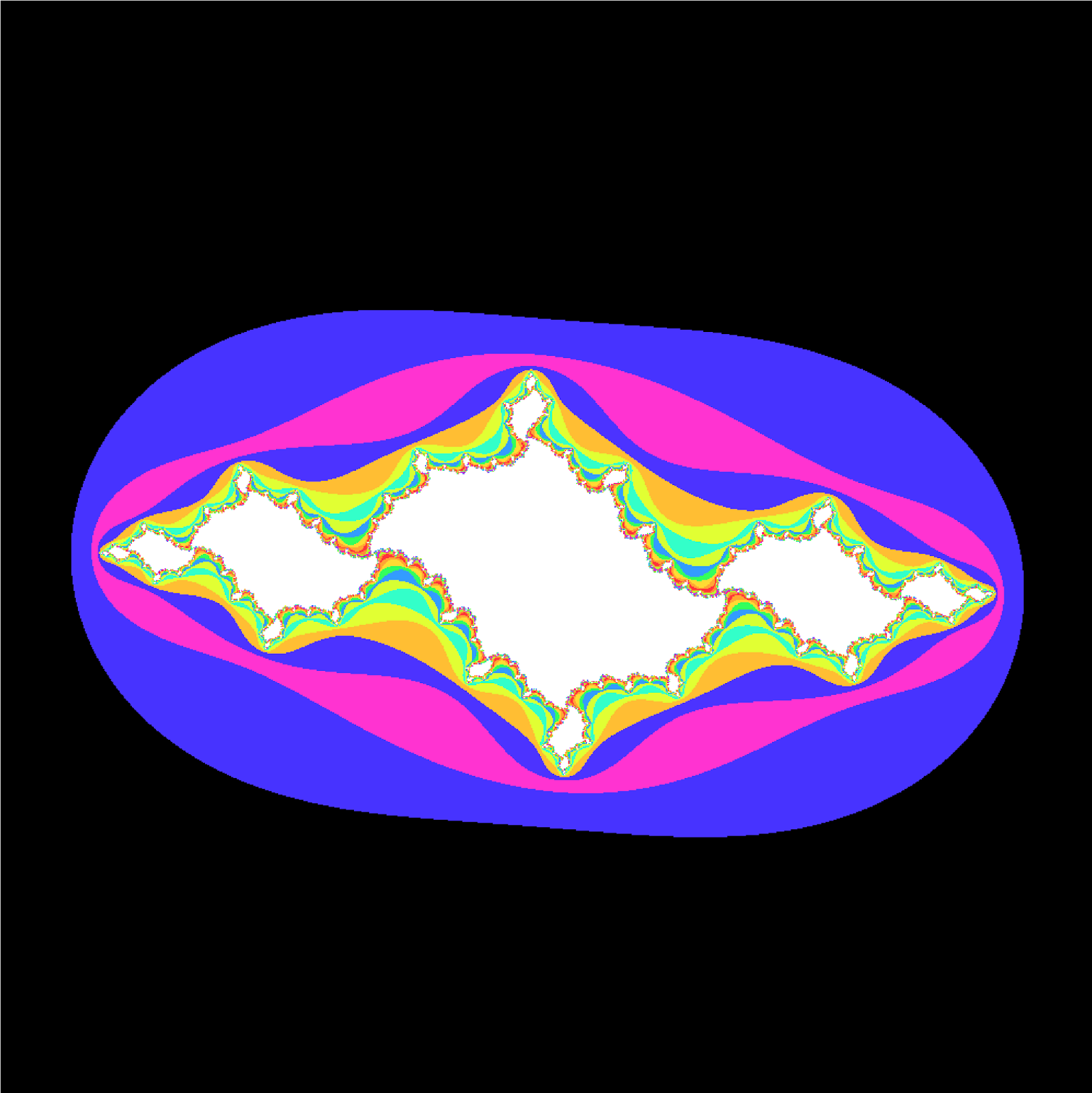
Adding colors: This is achieved by following the same process as above.

Sierpinski Gasket using Chaos game

#### Chaos game for generation of Sierpinski Gasket
# 1. Take 3 points in a plane to form a triangle, you need not draw it.
# 2. Randomly select any point inside the triangle and consider that your current position.
# 3. Randomly select any one of the 3 vertex points.
# 4. Move half the distance from your current position to the selected vertex.
# 5. Plot the current position.
# 6. Repeat from step 3

plot.new()
iterations <- 2000
vertices <- matrix(c(0,0,0.5,1,1,0),3,2, byrow=T)
current.point <- c(0.5,0.5)
random.vertex <- sample(1:3,iterations,replace=T)
plot.result = matrix(nrow=iterations,ncol=2)
for (i in 1:iterations){
 current.point <- (current.point+vertices[random.vertex[i],])/2
 plot.result[i,] <- current.point
}
points(plot.result,pch = 46)

Adding colors:

points(plot.result,pch = 46,col=c(13,3,41)[random.vertex])