[Paper Exploration] Deep Residual Learning for Image Recognition
Author: Kaiming He, Xiangyu Zhang, Shaoqing Ren, Jian Sun
Published on 2015
Abstract
Deeper neural networks are more difficult to train. We present a residual learning framework to ease the training of networks that are substantially deeper than those used previously. We explicitly reformulate the layers as learning residual functions with reference to the layer inputs, instead of learning unreferenced functions. We provide comprehensive empirical evidence showing that these residual networks are easier to optimize, and can gain accuracy from considerably increased depth. On the ImageNet dataset we evaluate residual nets with a depth of up to 152 layers—8x deeper than VGG nets but still having lower complexity. An ensemble of these residual nets achieves 3.57% error on the ImageNet test set. This result won the 1st place on the ILSVRC 2015 classification task. We also present analysis on CIFAR-10 with 100 and 1000 layers.
The depth of representations is of central importance for many visual recognition tasks. Solely due to our extremely deep representations, we obtain a 28% relative improvement on the COCO object detection dataset. Deep residual nets are foundations of our submissions to ILSVRC & COCO 2015 competitions, where we also won the 1st places on the tasks of ImageNet detection, ImageNet localization, COCO detection, and COCO segmentation.
Timeline
1943
Artificial Neurons: Warren McCulloch and Walter Pitts propose the first mathematical model of artificial neurons, laying the foundation for neural network theory. Their work introduces the concept of a simplified model of a neuron and its computational capabilities.
1958
Perceptron: Frank Rosenblatt develops the perceptron, a type of artificial neural network capable of learning simple patterns through supervised learning. It marks one of the first practical implementations of neural network concepts.
1960s-1970s
Neural Network Winter: Interest in neural networks declines due to the limitations of perceptrons, including their inability to solve non-linearly separable problems. This period sees reduced funding and research in neural network technologies.
1980
Neocognitron: Kunihiko Fukushima introduces the neocognitron, a hierarchical multilayered network designed for visual pattern recognition. It serves as a precursor to modern convolutional neural networks (CNNs).
1986
Backpropagation: David Rumelhart, Geoffrey Hinton, and Ronald Williams popularize backpropagation, an algorithm that enables the training of multilayer neural networks by efficiently calculating gradients and updating weights.
1998
LeNet-5: Yann LeCun et al. develop LeNet-5, a convolutional neural network designed for handwritten digit recognition. It demonstrates the practical effectiveness of CNNs and their potential in image classification tasks.
2006
Deep Belief Networks: Geoffrey Hinton et al. introduce deep belief networks, a type of deep neural network trained using unsupervised learning methods. This work marks a significant advancement in the deep learning era.
2012
AlexNet: Alex Krizhevsky, Ilya Sutskever, and Geoffrey Hinton win the ImageNet Large Scale Visual Recognition Challenge (ILSVRC) with AlexNet. This deep convolutional neural network achieves a dramatic improvement in image classification performance and sparks widespread adoption of deep learning.
2014
VGGNet: Karen Simonyan and Andrew Zisserman introduce VGGNet, which further deepens CNN architectures with a consistent design. VGGNet achieves state-of-the-art performance on ImageNet and influences subsequent network designs.
2015
ResNet: Kaiming He et al. introduce Residual Networks (ResNet), a groundbreaking architecture that allows for training extremely deep networks (over 100 layers) by using residual connections to address the vanishing gradient problem.
2016
DenseNet: Gao Huang et al. introduce DenseNet, which improves gradient flow and network efficiency by connecting each layer to every other layer in a feed-forward fashion, thereby enhancing feature reuse and reducing the number of parameters.
2017
Transformer: Ashish Vaswani et al. introduce the Transformer architecture in "Attention Is All You Need," revolutionizing natural language processing by relying solely on self-attention mechanisms, leading to improved performance in various NLP tasks.
2018
BERT: Jacob Devlin et al. introduce BERT (Bidirectional Encoder Representations from Transformers), which achieves state-of-the-art results on a range of NLP tasks by pre-training deep bidirectional representations and fine-tuning on specific tasks.
2019
EfficientNet: Mingxing Tan and Quoc V. Le introduce EfficientNet, a family of models that use a compound scaling method to optimize the balance between network depth, width, and resolution, improving both efficiency and accuracy.
2020
GPT-3: OpenAI releases GPT-3 (Generative Pre-trained Transformer 3), a language model with 175 billion parameters. GPT-3 demonstrates impressive capabilities in generating coherent and contextually relevant text across diverse applications.
2021
Vision Transformer (ViT): Alexey Dosovitskiy et al. introduce Vision Transformers, applying the Transformer architecture to image recognition tasks and achieving competitive performance with traditional CNNs by leveraging self-attention mechanisms.
2022
DALL-E 2: OpenAI releases DALL-E 2, an advanced generative model capable of creating highly realistic images from textual descriptions, showcasing the power of combining transformers with generative modeling.
2023
Further Advancements: Continued research and development in neural networks, with ongoing improvements in model efficiency, interpretability, and applications across various domains, including healthcare, autonomous systems, and beyond.
Glossary
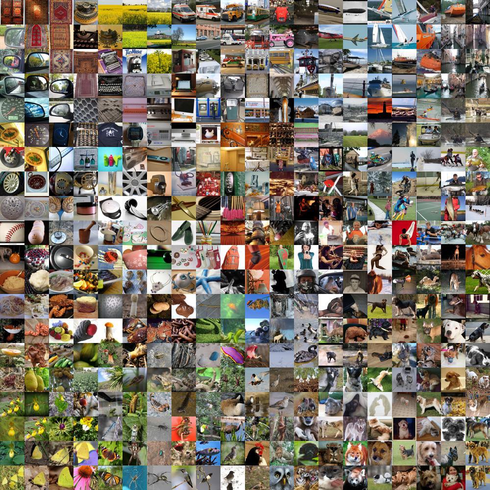
ImageNet:
A large visual database used for visual object recognition software research. It is a benchmark dataset in computer vision, consisting of millions of labeled images categorized into thousands of classes.
PASCAL and MS COCO
PASCAL Visual Object Classes (VOC):
- Purpose: The PASCAL VOC dataset is designed for object recognition and detection tasks.
- Content: It contains images from various categories, such as people, animals, and vehicles. The dataset includes annotations for object classes, bounding boxes, and segmentation masks.
- Challenges: The dataset is known for the PASCAL VOC challenges, which are annual competitions that focus on evaluating the performance of different algorithms on object detection, classification, and segmentation tasks.
- Categories: There are 20 object classes in PASCAL VOC, such as person, bicycle, bird, cat, cow, and more.
- Usage: It is widely used for benchmarking and training models in object detection and segmentation tasks.

Microsoft Common Objects in Context (COCO):
- Purpose: The MS COCO dataset is used for a variety of computer vision tasks, including object detection, segmentation, keypoint detection, and image captioning.
- Content: It contains a large number of images with objects in natural and complex scenes, along with annotations for object classes, segmentation masks, keypoints (for human pose estimation), and image captions.
- Challenges: The COCO challenges, held annually, evaluate models on tasks such as object detection, instance segmentation, and image captioning.
- Categories: There are 80 object categories in COCO, such as person, bicycle, car, dog, bottle, and more.
- Usage: COCO is one of the most comprehensive and widely used datasets in computer vision, known for its diversity and the complexity of its scenes. It is used for training and benchmarking models across various tasks.

State-of-the-Art (SOTA):
Refers to the highest level of development or the best performance achieved in a particular field at a given time.
VGG Nets
VGG nets are a type of convolutional neural network architecture known for their simplicity and depth. Developed by the Visual Geometry Group at the University of Oxford, VGG networks consist of very small (3x3) convolution filters and are characterized by their uniform architecture. They have been widely used in image recognition tasks.

*
Degradation Problem
The degradation problem in deep learning refers to the phenomenon where adding more layers to a deep neural network leads to a higher training error and test error, contrary to what one might expect. This issue arises due to difficulties in training very deep networks.
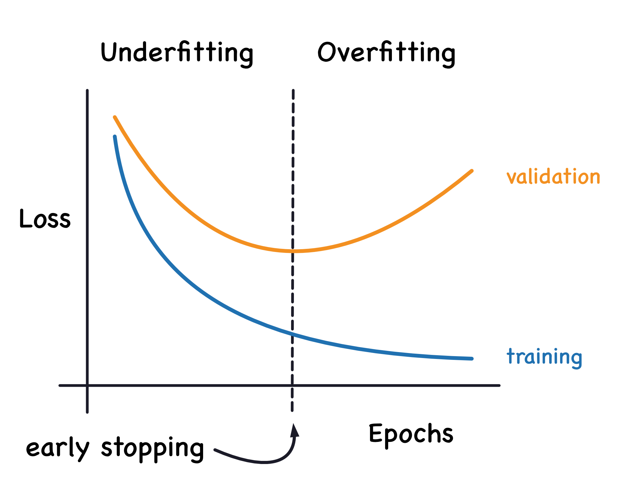
Overfitting
Overfitting occurs when a machine learning model learns the training data too well, including the noise and outliers, leading to poor performance on new, unseen data. This happens when the model is too complex relative to the amount of training data.
Identity Mapping
Identity mapping is a technique used in neural networks, particularly in residual networks, where the input to a layer is passed directly to a subsequent layer without any transformation. This helps in addressing the degradation problem by ensuring that layers can learn identity mappings if they do not improve the objective.
mAP
mAP (mean Average Precision) is a metric used to evaluate the accuracy of object detection models. It is the mean of the average precision scores for each class, providing a single number that reflects the model’s ability to detect objects of various classes.

Vanishing Gradient Problem:
A difficulty encountered during the training of deep neural networks, where the gradients of the loss function with respect to the parameters become very small, effectively preventing the weights from updating.

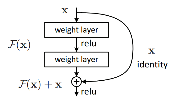
Residual Block
A residual block is a fundamental component of residual neural networks (ResNets) designed to solve the degradation problem by allowing the network to skip one or more layers. The input to a residual block is added to the output of the block’s layers, which helps in training very deep networks.
Bottleneck Residual Block
A bottleneck residual block is a variation of the residual block used in deep residual networks to reduce the number of parameters and computation. It consists of three layers: a 1x1 convolution that reduces the dimensions, a 3x3 convolution, and another 1x1 convolution that restores the dimensions. This structure helps in making the network deeper while keeping the computational cost manageable.
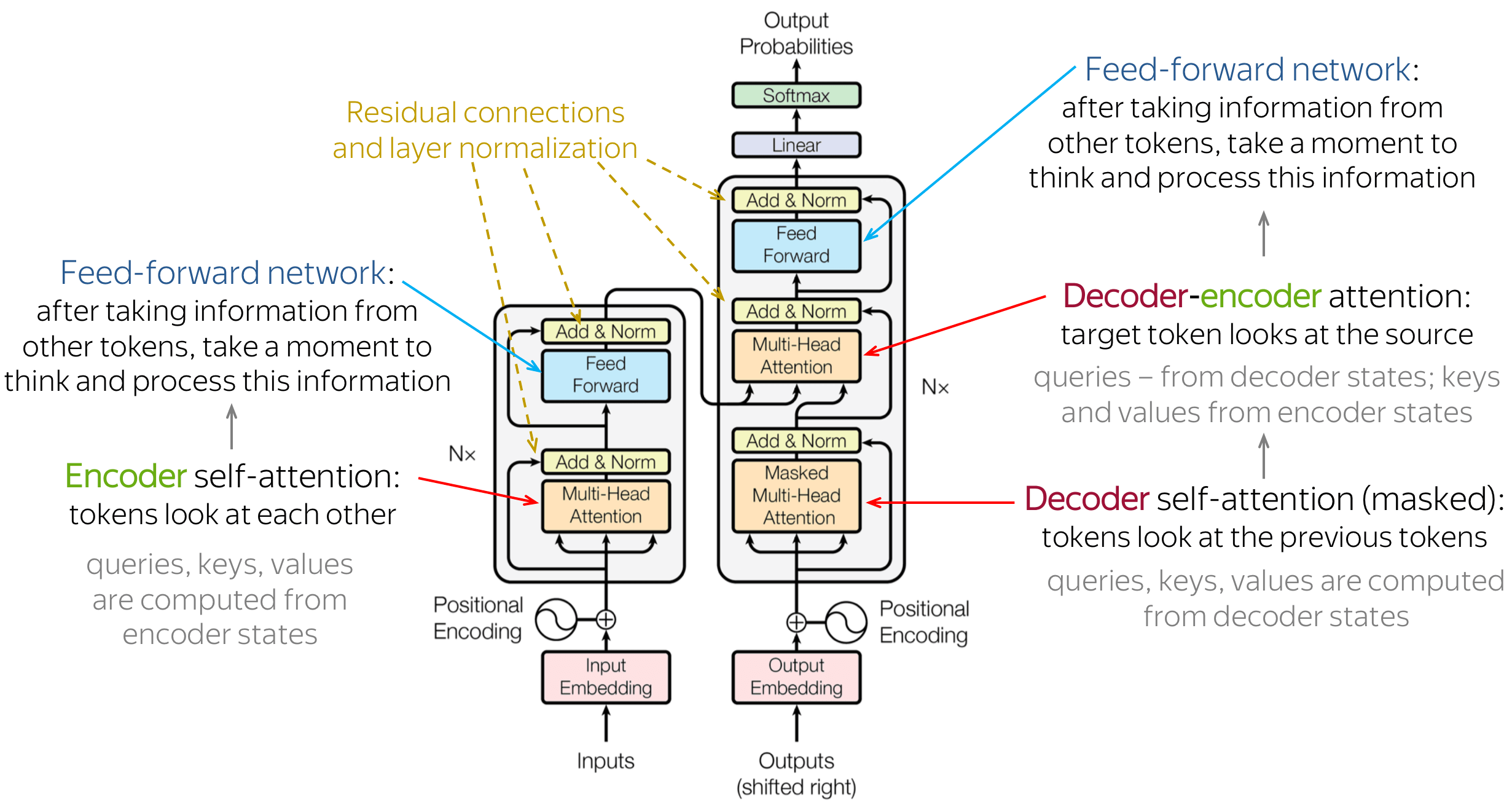
Transformer Block
A transformer block is a key component of the transformer architecture, used extensively in natural language processing tasks. It consists of a multi-head self-attention mechanism followed by a position-wise feed-forward network. This architecture allows the model to capture complex dependencies in the data.
Core concepts
Introduction
- Objective: To address the degradation problem in deep neural networks and improve image recognition performance.
- Degradation Problem: As the depth of neural networks increases, accuracy saturates and then degrades.
Methodology
Residual Learning
- Introduced the concept of residual learning to facilitate the training of deep networks.
- Residual Block:
- Consists of a series of layers where the input is directly added to the output of the stacked layers.
- Formulated as: $y = \mathcal{F}(x, {W_i}) + x$ where $(\mathcal{F}(x, {W_i}))$ represents the residual mapping.
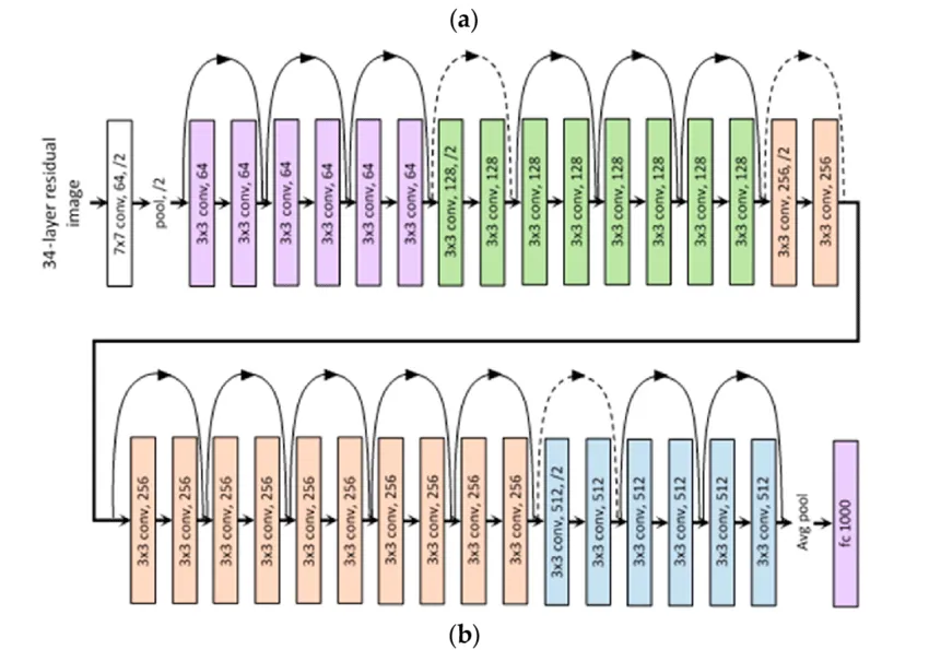
Architecture
ResNet Architecture
- Built networks with depths of 34, 50, 101, and 152 layers.
- Demonstrated significant improvements over traditional networks.
Bottleneck Design
- Used for deeper architectures.
- Consists of three layers:
- 1x1 convolutions
- 3x3 convolutions
- 1x1 convolutions

Experiments and Results
Datasets
- Evaluated on ImageNet, CIFAR-10, and COCO.
ImageNet Results
- Achieved top-5 error rates of 3.57% and 3.6% with 152-layer and 101-layer ResNets, respectively.
- ResNet-152 outperformed VGG-19 by 8.4%.
COCO Detection
- Integrated with Faster R-CNN.
- Achieved improvements in object detection and segmentation tasks.
Generalization
- Demonstrated that residual networks generalize well across various datasets and tasks.
Insights
Vanishing Gradient
- Residual learning mitigates the vanishing gradient problem, allowing deeper networks to be trained.
Ease of Optimization
- Residual networks are easier to optimize than their plain counterparts.
Identity Mapping
- Identity shortcuts help in retaining the essential identity mappings in the networks.
Conclusion
Impact
- Residual networks have become a standard in deep learning, influencing subsequent research and applications.
- Demonstrated the ability to train extremely deep networks without performance degradation.
Future Work
- Suggested exploring the integration of residual learning with other network architectures and tasks.
Supplementary Contributions
Residual Blocks Variants
- Investigated different variants of residual blocks to study their effects on performance.
Training Strategies
- Discussed training strategies to efficiently train deep networks with residual blocks.
Key Takeaways
- Residual learning allows for the effective training of very deep networks.
- ResNets significantly improve performance across various image recognition tasks.
- The methodology can be generalized to other domains and applications in deep learning.
Pytorch Implementation
import torch
import torch.nn as nn
import torchvision
import torchvision.transforms as transforms
from torch.utils.data import DataLoader
from torch.backends import cudnn
import time

cudnn.benchmark = True
use_cuda = torch.cuda.is_available()

# Image Preprocessing
transform = transforms.Compose([
    transforms.Resize(40),
    transforms.RandomHorizontalFlip(),
    transforms.RandomCrop(32),
    transforms.ToTensor()
])

# CIFAR-10 Dataset
train_dataset = torchvision.datasets.CIFAR10(root='./data', train=True, transform=transform, download=True)
test_dataset = torchvision.datasets.CIFAR10(root='./data', train=False, transform=transforms.ToTensor())

# Data Loader
train_loader = DataLoader(dataset=train_dataset, batch_size=100, shuffle=True)
test_loader = DataLoader(dataset=test_dataset, batch_size=100, shuffle=False)

# Simple CNN Model
class SimpleCNN(nn.Module):
    def __init__(self, num_classes=10):
        super(SimpleCNN, self).__init__()
        self.layer1 = nn.Sequential(
            nn.Conv2d(3, 16, kernel_size=5, padding=2),
            nn.BatchNorm2d(16),
            nn.ReLU(),
            nn.MaxPool2d(kernel_size=2, stride=2)
        )
        self.layer2 = nn.Sequential(
            nn.Conv2d(16, 32, kernel_size=5, padding=2),
            nn.BatchNorm2d(32),
            nn.ReLU(),
            nn.MaxPool2d(kernel_size=2, stride=2)
        )
        self.fc = nn.Linear(32 * 8 * 8, num_classes)

    def forward(self, x):
        out = self.layer1(x)
        out = self.layer2(out)
        out = out.view(out.size(0), -1)
        out = self.fc(out)
        return out

# Residual Block
def conv3x3(in_channels, out_channels, stride=1):
    """3x3 convolution with padding"""
    return nn.Conv2d(in_channels, out_channels, kernel_size=3, stride=stride, padding=1, bias=False)

class ResidualBlock(nn.Module):
    def __init__(self, in_channels, out_channels, stride=1, downsample=None):
        super(ResidualBlock, self).__init__()
        self.conv1 = conv3x3(in_channels, out_channels, stride)
        self.bn1 = nn.BatchNorm2d(out_channels)
        self.relu = nn.ReLU(inplace=True)
        self.conv2 = conv3x3(out_channels, out_channels)
        self.bn2 = nn.BatchNorm2d(out_channels)
        self.downsample = downsample

    def forward(self, x):
        residual = x
        out = self.conv1(x)
        out = self.bn1(out)
        out = self.relu(out)
        out = self.conv2(out)
        out = self.bn2(out)
        if self.downsample:
            residual = self.downsample(x)
        out += residual
        out = self.relu(out)
        return out

# ResNet Model
class ResNet(nn.Module):
    def __init__(self, block, layers, num_classes=10):
        super(ResNet, self).__init__()
        self.in_channels = 16
        self.conv = conv3x3(3, 16)
        self.bn = nn.BatchNorm2d(16)
        self.relu = nn.ReLU(inplace=True)
        self.layer1 = self.make_layer(block, 16, layers[0])
        self.layer2 = self.make_layer(block, 32, layers[1], 2)
        self.layer3 = self.make_layer(block, 64, layers[2], 2)
        self.avg_pool = nn.AvgPool2d(8)
        self.fc = nn.Linear(64, num_classes)

    def make_layer(self, block, out_channels, blocks, stride=1):
        downsample = None
        if (stride != 1) or (self.in_channels != out_channels):
            downsample = nn.Sequential(
                conv3x3(self.in_channels, out_channels, stride),
                nn.BatchNorm2d(out_channels)
            )
        layers = []
        layers.append(block(self.in_channels, out_channels, stride, downsample))
        self.in_channels = out_channels
        for i in range(1, blocks):
            layers.append(block(out_channels, out_channels))
        return nn.Sequential(*layers)

    def forward(self, x):
        out = self.conv(x)
        out = self.bn(out)
        out = self.relu(out)  # 32 x 32 x 16
        out = self.layer1(out)  # 32 x 32 x 16
        out = self.layer2(out)  # 16 x 16 x 32
        out = self.layer3(out)  # 8 x 8 x 64
        out = self.avg_pool(out)  # 1 x 1 x 64
        out = out.view(out.size(0), -1)  # None x 64
        out = self.fc(out)  # None x 10
        return out

# Initialize models
device = torch.device("cuda" if torch.cuda.is_available() else "cpu")
simple_cnn = SimpleCNN().to(device)
resnet = ResNet(ResidualBlock, [2, 2, 2]).to(device)

# Loss and optimizer
criterion = nn.CrossEntropyLoss()
optimizer_simple_cnn = torch.optim.Adam(simple_cnn.parameters(), lr=0.001)
optimizer_resnet = torch.optim.Adam(resnet.parameters(), lr=0.001)

"""Resnet"""

# Training function
def train(model, optimizer, num_epochs=10):
    model.train()
    for epoch in range(num_epochs):
        running_loss = 0.0
        for i, (images, labels) in enumerate(train_loader):
            images, labels = images.to(device), labels.to(device)

            # Forward pass
            outputs = model(images)
            loss = criterion(outputs, labels)

            # Backward and optimize
            optimizer.zero_grad()
            loss.backward()
            optimizer.step()

            running_loss += loss.item()

            if (i + 1) % 100 == 0:
                print(f'Epoch [{epoch + 1}/{num_epochs}], Step [{i + 1}/{len(train_loader)}], Loss: {loss.item():.4f}')
        print(f'Epoch [{epoch + 1}/{num_epochs}], Loss: {running_loss / len(train_loader):.4f}')

# Testing function
def test(model):
    model.eval()
    correct = 0
    total = 0
    with torch.no_grad():
        for images, labels in test_loader:
            images, labels = images.to(device), labels.to(device)
            outputs = model(images)
            _, predicted = torch.max(outputs.data, 1)
            total += labels.size(0)
            correct += (predicted == labels).sum().item()
    print(f'Accuracy of the model on the 10000 test images: {100 * correct / total:.2f}%')

# Train and test SimpleCNN
print("Training SimpleCNN")
train(simple_cnn, optimizer_simple_cnn)
print("Testing SimpleCNN")
test(simple_cnn)

# Train and test ResNet
print("Training ResNet")
train(resnet, optimizer_resnet)
print("Testing ResNet")
test(resnet)
Results
Training SimpleCNN
Epoch [1/10], Step [100/500], Loss: 1.2978
Epoch [1/10], Step [200/500], Loss: 1.3175
Epoch [1/10], Step [300/500], Loss: 1.1620
Epoch [1/10], Step [400/500], Loss: 1.1292
Epoch [1/10], Step [500/500], Loss: 1.1444
Epoch [1/10], Loss: 1.2770
Epoch [2/10], Step [100/500], Loss: 1.0181
Epoch [2/10], Step [200/500], Loss: 1.0906
Epoch [2/10], Step [300/500], Loss: 0.9453
Epoch [2/10], Step [400/500], Loss: 1.1281
Epoch [2/10], Step [500/500], Loss: 1.1890
Epoch [2/10], Loss: 1.1697
Epoch [3/10], Step [100/500], Loss: 0.9400
Epoch [3/10], Step [200/500], Loss: 1.0746
Epoch [3/10], Step [300/500], Loss: 1.0551
Epoch [3/10], Step [400/500], Loss: 1.0406
Epoch [3/10], Step [500/500], Loss: 0.9414
Epoch [3/10], Loss: 1.1119
Epoch [4/10], Step [100/500], Loss: 0.9787
Epoch [4/10], Step [200/500], Loss: 1.1228
Epoch [4/10], Step [300/500], Loss: 1.0656
Epoch [4/10], Step [400/500], Loss: 0.8739
Epoch [4/10], Step [500/500], Loss: 0.9911
Epoch [4/10], Loss: 1.0867
Epoch [5/10], Step [100/500], Loss: 1.1093
Epoch [5/10], Step [200/500], Loss: 1.0494
Epoch [5/10], Step [300/500], Loss: 1.1796
Epoch [5/10], Step [400/500], Loss: 1.1727
Epoch [5/10], Step [500/500], Loss: 0.8257
Epoch [5/10], Loss: 1.0568
Epoch [6/10], Step [100/500], Loss: 1.1401
Epoch [6/10], Step [200/500], Loss: 0.9372
Epoch [6/10], Step [300/500], Loss: 0.9893
Epoch [6/10], Step [400/500], Loss: 0.7880
Epoch [6/10], Step [500/500], Loss: 0.9031
Epoch [6/10], Loss: 1.0365
Epoch [7/10], Step [100/500], Loss: 1.2074
Epoch [7/10], Step [200/500], Loss: 0.9227
Epoch [7/10], Step [300/500], Loss: 1.0585
Epoch [7/10], Step [400/500], Loss: 1.0177
Epoch [7/10], Step [500/500], Loss: 1.0659
Epoch [7/10], Loss: 1.0098
Epoch [8/10], Step [100/500], Loss: 0.9883
Epoch [8/10], Step [200/500], Loss: 0.9500
Epoch [8/10], Step [300/500], Loss: 0.9642
Epoch [8/10], Step [400/500], Loss: 0.8540
Epoch [8/10], Step [500/500], Loss: 1.0021
Epoch [8/10], Loss: 0.9926
Epoch [9/10], Step [100/500], Loss: 0.9815
Epoch [9/10], Step [200/500], Loss: 1.0014
Epoch [9/10], Step [300/500], Loss: 0.9835
Epoch [9/10], Step [400/500], Loss: 0.8745
Epoch [9/10], Step [500/500], Loss: 0.9122
Epoch [9/10], Loss: 0.9786
Epoch [10/10], Step [100/500], Loss: 1.1003
Epoch [10/10], Step [200/500], Loss: 0.9819
Epoch [10/10], Step [300/500], Loss: 1.0853
Epoch [10/10], Step [400/500], Loss: 1.0723
Epoch [10/10], Step [500/500], Loss: 0.7785
Epoch [10/10], Loss: 0.9672
Testing SimpleCNN
Accuracy of the model on the 10000 test images: 62.53%
Training ResNet
Epoch [1/10], Step [100/500], Loss: 1.1892
Epoch [1/10], Step [200/500], Loss: 1.0114
Epoch [1/10], Step [300/500], Loss: 1.0300
Epoch [1/10], Step [400/500], Loss: 0.9715
Epoch [1/10], Step [500/500], Loss: 1.0377
Epoch [1/10], Loss: 1.0426
Epoch [2/10], Step [100/500], Loss: 0.8975
Epoch [2/10], Step [200/500], Loss: 0.9486
Epoch [2/10], Step [300/500], Loss: 0.9703
Epoch [2/10], Step [400/500], Loss: 0.8699
Epoch [2/10], Step [500/500], Loss: 0.7683
Epoch [2/10], Loss: 0.8947
Epoch [3/10], Step [100/500], Loss: 0.7991
Epoch [3/10], Step [200/500], Loss: 0.7637
Epoch [3/10], Step [300/500], Loss: 0.8086
Epoch [3/10], Step [400/500], Loss: 0.6720
Epoch [3/10], Step [500/500], Loss: 0.6858
Epoch [3/10], Loss: 0.7990
Epoch [4/10], Step [100/500], Loss: 0.7963
Epoch [4/10], Step [200/500], Loss: 0.7246
Epoch [4/10], Step [300/500], Loss: 0.5814
Epoch [4/10], Step [400/500], Loss: 0.8705
Epoch [4/10], Step [500/500], Loss: 0.7726
Epoch [4/10], Loss: 0.7340
Epoch [5/10], Step [100/500], Loss: 0.7007
Epoch [5/10], Step [200/500], Loss: 0.7134
Epoch [5/10], Step [300/500], Loss: 0.6847
Epoch [5/10], Step [400/500], Loss: 0.8029
Epoch [5/10], Step [500/500], Loss: 0.6260
Epoch [5/10], Loss: 0.6778
Epoch [6/10], Step [100/500], Loss: 0.8832
Epoch [6/10], Step [200/500], Loss: 0.6445
Epoch [6/10], Step [300/500], Loss: 0.6671
Epoch [6/10], Step [400/500], Loss: 0.4728
Epoch [6/10], Step [500/500], Loss: 0.7115
Epoch [6/10], Loss: 0.6414
Epoch [7/10], Step [100/500], Loss: 0.7021
Epoch [7/10], Step [200/500], Loss: 0.7717
Epoch [7/10], Step [300/500], Loss: 0.4920
Epoch [7/10], Step [400/500], Loss: 0.6622
Epoch [7/10], Step [500/500], Loss: 0.5240
Epoch [7/10], Loss: 0.6059
Epoch [8/10], Step [100/500], Loss: 0.5715
Epoch [8/10], Step [200/500], Loss: 0.5650
Epoch [8/10], Step [300/500], Loss: 0.4841
Epoch [8/10], Step [400/500], Loss: 0.7781
Epoch [8/10], Step [500/500], Loss: 0.4514
Epoch [8/10], Loss: 0.5774
Epoch [9/10], Step [100/500], Loss: 0.4952
Epoch [9/10], Step [200/500], Loss: 0.4070
Epoch [9/10], Step [300/500], Loss: 0.5137
Epoch [9/10], Step [400/500], Loss: 0.4824
Epoch [9/10], Step [500/500], Loss: 0.5795
Epoch [9/10], Loss: 0.5528
Epoch [10/10], Step [100/500], Loss: 0.4072
Epoch [10/10], Step [200/500], Loss: 0.6239
Epoch [10/10], Step [300/500], Loss: 0.5173
Epoch [10/10], Step [400/500], Loss: 0.4408
Epoch [10/10], Step [500/500], Loss: 0.5978
Epoch [10/10], Loss: 0.5323
Testing ResNet
Accuracy of the model on the 10000 test images: 70.57%
GPT Quiz
1. What is the primary motivation behind the development of ResNet?
- a) To improve the computational efficiency of CNNs
- b) To address the problem of vanishing gradients in deep networks
- c) To introduce new types of activation functions
- d) To reduce the memory footprint of neural networks
2. What is a “residual block” in the context of ResNet?
- a) A standard convolutional block with batch normalization
- b) A block with convolutional layers followed by a fully connected layer
- c) A block with a shortcut connection that bypasses one or more layers
- d) A block that only contains ReLU activation functions
3. What is the main advantage of using residual connections in deep networks?
- a) They reduce the number of parameters
- b) They make the network more interpretable
- c) They allow for the training of much deeper networks by mitigating the vanishing gradient problem
- d) They decrease the overall training time
4. In ResNet, what does the shortcut connection typically do in terms of computation?
- a) It performs a downsampling operation
- b) It adds the output of a residual block to the input
- c) It multiplies the output of a residual block by a constant
- d) It passes the input through a fully connected layer
5. How did ResNet perform on the ImageNet classification task compared to previous models?
- a) It achieved lower accuracy but with fewer parameters
- b) It achieved higher accuracy and won the ILSVRC 2015 competition
- c) It had similar accuracy but was faster to train
- d) It underperformed compared to VGGNet
6. What is the depth of the deepest ResNet model discussed in the original paper?
- a) 34 layers
- b) 50 layers
- c) 101 layers
- d) 152 layers
7. What kind of operation is used in ResNet to deal with the increasing depth of the network?
- a) Max pooling
- b) Average pooling
- c) Batch normalization
- d) Gradient clipping
8. Which of the following techniques is NOT used in the original ResNet architecture?
- a) Batch normalization
- b) ReLU activation
- c) Dropout
- d) Shortcut connections
9. What kind of problem did the authors demonstrate ResNet could solve more effectively than traditional deep networks?
- a) Object detection
- b) Semantic segmentation
- c) Image classification on very deep networks
- d) Language modeling
10. What was a key architectural innovation that distinguished ResNet from previous deep convolutional networks?
- a) The use of 3x3 convolutions
- b) The introduction of residual learning with identity mappings
- c) The integration of attention mechanisms
- d) The use of LSTM layers
11. How does ResNet address the degradation problem in deep networks?
- a) By reducing the learning rate
- b) By adding more fully connected layers
- c) By introducing residual connections that help optimize the network
- d) By using smaller convolutional filters
12. Which of the following statements is true about the identity mapping in ResNet?
- a) It multiplies the input by a constant factor
- b) It passes the input through an additional convolutional layer
- c) It skips a layer by adding the input directly to the output of the next layer
- d) It subtracts the input from the output of the layer
13. What is the main benefit of using deeper ResNet models like ResNet-152?
- a) They achieve lower accuracy but are more computationally efficient
- b) They improve the representation learning capability, leading to better performance on complex tasks
- c) They require less memory compared to shallower models
- d) They eliminate the need for data augmentation
14. What type of skip connection is used in the original ResNet architecture?
- a) Concatenation of input and output
- b) Element-wise multiplication of input and output
- c) Element-wise addition of input and output
- d) Concatenation followed by a convolutional layer
15. In ResNet, what is the role of the 1x1 convolution in the bottleneck architecture?
- a) To reduce dimensionality
- b) To increase the receptive field
- c) To add non-linearity
- d) To perform max pooling
16. Which of the following is a characteristic of the ResNet bottleneck architecture?
- a) It uses a single 3x3 convolution per block
- b) It uses a sequence of 1x1, 3x3, and 1x1 convolutions
- c) It removes batch normalization from the network
- d) It avoids using any non-linear activation functions
17. What is the primary reason for using a bottleneck design in deeper ResNet models?
- a) To reduce the number of parameters while maintaining model capacity
- b) To simplify the training process
- c) To increase the number of activations per layer
- d) To avoid overfitting
18. In ResNet, how are shortcut connections typically implemented when the dimensions of the input and output differ?
- a) By using average pooling
- b) By adding zero-padding to the input
- c) By using a 1x1 convolution to match dimensions
- d) By ignoring the input and only using the output
19. What problem does the “vanishing gradient” refer to in the context of training deep neural networks?
- a) Gradients become too large, leading to instability during training
- b) Gradients become too small, causing slow convergence and difficulty in training deep networks
- c) The loss function does not converge
- d) The network fails to generalize to new data
20. How does ResNet compare with VGGNet in terms of network depth and performance?
- a) ResNet is shallower and less accurate than VGGNet
- b) ResNet is deeper and more accurate than VGGNet
- c) ResNet is deeper but less accurate than VGGNet
- d) ResNet is similar in depth but more accurate than VGGNet
Sources:
- Krizhevsky, A., Sutskever, I., & Hinton, G. E. (2012). “ImageNet classification with deep convolutional neural networks.” Advances in Neural Information Processing Systems, 25, 1097-1105.
- Everingham, M., Van Gool, L., Williams, C. K. I., Winn, J., & Zisserman, A. (2010). “The Pascal Visual Object Classes (VOC) challenge.” International Journal of Computer Vision, 88(2), 303-338.
- Lin, T. Y., Maire, M., Belongie, S., Hays, J., Perona, P., Ramanan, D., … & Zitnick, C. L. (2014). “Microsoft COCO: Common objects in context.” European Conference on Computer Vision, 740-755.
- Glorot, X., Bordes, A., & Bengio, Y. (2011). “Deep sparse rectifier neural networks.” Proceedings of the Fourteenth International Conference on Artificial Intelligence and Statistics, 315-323.
- Simonyan, K., & Zisserman, A. (2015). “Very deep convolutional networks for large-scale image recognition.” International Conference on Learning Representations.
- He, K., Zhang, X., Ren, S., & Sun, J. (2016). “Deep residual learning for image recognition.” Proceedings of the IEEE Conference on Computer Vision and Pattern Recognition, 770-778.
- Papers with Code. “ImageNet.” Retrieved from https://production-media.paperswithcode.com/datasets/ImageNet-0000000008-f2e87edd_Y0fT5zg.jpg
- ResearchGate. “Concepts of the PASCAL Visual Object Challenge 2007.” Retrieved from https://www.researchgate.net/publication/221368944/figure/fig4/AS:668838140067847@1536474847482/Concepts-of-the-PASCAL-Visual-Object-Challenge-2007-used-in-the-image-benchmark-of.png
- ResearchGate. “Sample images from the COCO dataset.” Retrieved from https://www.researchgate.net/publication/344601010/figure/fig3/AS:945595862745089@1602459030487/Sample-images-from-the-COCO-dataset.png
- LinkedIn. “Forward Propagation.” Retrieved from https://media.licdn.com/dms/image/D5612AQGNjUevxbUE_A/article-cover_image-shrink_720_1280/0/1677211887007?e=1728518400&v=beta&t=5If5-6JzeWUD_QoyivK3Q0l10oelax0NVqTdj8OIYDk
- Medium. “ReLU Function.” Retrieved from https://miro.medium.com/v2/resize:fit:1400/1*XxxiA0jJvPrHEJHD4z893g.png
- Papers with Code. “VGG Net.” Retrieved from https://production-media.paperswithcode.com/methods/vgg_7mT4DML.png
- Kaggle. “Overfitting.” Retrieved from https://storage.googleapis.com/kaggle-media/learn/images/eP0gppr.png
- AIML.com. “Vanishing and Exploding Gradient.” Retrieved from https://aiml.com/wp-content/uploads/2023/11/vanishing-and-exploding-gradient-1.png
- GitHub. “mAP Formula.” Retrieved from https://cdn.prod.website-files.com/614c82ed388d53640613982e/64876df5c42ecf0cf93f549d_mean%20average%20precision%20formula.webp
- Quora. “Degradation Problem in Neural Networks.” Retrieved from https://qph.cf2.quoracdn.net/main-qimg-e148d117f06700fbc474f425c01e3f5e-pjlq
- Medium. “Residual Block.” Retrieved from https://miro.medium.com/v2/resize:fit:570/1*D0F3UitQ2l5Q0Ak-tjEdJg.png
- Medium. “ResNet Architecture.” Retrieved from https://miro.medium.com/v2/resize:fit:1400/format:webp/1*C8jf92MeHZnxnbpMkz6jkQ.png
- Stack Exchange. “Bottleneck Design.” Retrieved from https://i.sstatic.net/kbiIG.png
- Resnet Code from this github gist