Sampling Methodology
Sampling is the process of selecting a subset from a larger population to make inferences about the whole. Basically, it allows us to estimate characteristics of the whole population by examining only a part of it.
Example: We have 1000 student assignments. Instead of reviewing all, we sample a subset to infer the quality of all assignments.
Types of Sampling Methods
Probability Sampling

-
Simple Random Sampling: Every item has an equal chance of being selected.
We use a random number generator to pick 50 assignments out of 1000.
-
Systematic Sampling: Select every nth item from a list.
We choose every 20th assignment from a list of 1000.
-
Stratified Sampling: Divide the population into strata and sample from each.
We group by assignment type (e.g., essays, quizzes) and sample from each group.
-
Cluster Sampling: Divide into clusters, then sample entire clusters.
We randomly select a few classes and review all assignments from those classes.
Non-Probability Sampling
-
Convenience Sampling: Select items that are easiest to access.
We review assignments from students who submitted them early.
-
Judgmental Sampling: Use expert judgment to select representative items.
We choose assignments of varying difficulty levels.
Sample Size Determination
Desired confidence level, margin of error, and population size.
Confidence Level
The confidence level is the probability that the confidence interval contains the true population parameter. It reflects the certainty that the true parameter is captured by the sample’s estimate.
If we select a confidence level of 95%, this means we are 95% confident that the true proportion of errors in all student assignments is within our sample’s calculated range.
Margin of Error (E)
The margin of error is the range within which the true population parameter is expected to lie, given the confidence level. It represents the uncertainty associated with the sample estimate.
If the estimated proportion of assignments with errors is 60% and the margin of error is ±5%, then the true proportion of assignments with errors is expected to be between 55% and 65%.
$E = Z \times \sqrt{\frac{p(1 - p)}{n}}$
Z-Score
The z-score corresponds to the critical value from the standard normal distribution for a given confidence level. It indicates how many standard deviations a point is from the mean.
For a 95% confidence level, the z-score is 1.96. This means that 95% of the possible sample estimates lie within 1.96 standard deviations of the true proportion of assignments with errors.
For 90% confidence: $Z = 1.645$
For 95% confidence: $Z = 1.96$
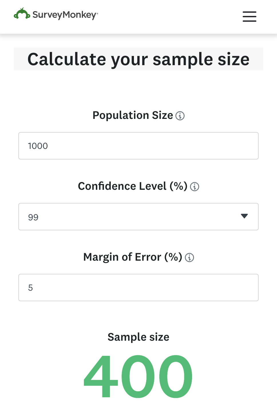
For 99% confidence: $Z = 2.576$
Proportion (p)
Worst-Case Scenario (Unknown Case)
When the true population proportion is unknown, the most conservative estimate assumes $p = 0.5$, maximizing variability and resulting in the largest required sample size.
If we have no prior information about the proportion of student assignments with errors, we assume $p = 0.5$ to account for the highest uncertainty.
Known Case
When the population proportion is known or estimated from prior studies, this value can be directly used in sample size calculations.
If previous data shows that 40% of assignments contain errors, we use $p = 0.4$ to calculate a more specific sample size.
Sample Size Formula
The sample size needed to estimate a population proportion with a desired confidence level and margin of error can be calculated as:
$$ n = \frac{Z^2 \cdot p(1 - p)}{E^2} $$
Where:
- $n$ is the sample size
- $Z$ is the z-score corresponding to the confidence level
- $p$ is the estimated population proportion
- $E$ is the margin of error
To estimate the proportion of assignments with errors with a 95% confidence level ($Z = 1.96$) and a margin of error of 5% ($E = 0.05$), assuming no prior knowledge about the proportion ($p = 0.5$), the required sample size would be:
$$ n = \frac{(1.96)^2 \cdot 0.5(1 - 0.5)}{(0.05)^2} = 384.16 $$
This means we would need to sample approximately 385 student assignments. However, this does not account for population size because it is typically used when the population is infinite or very large. In such cases, the effect of population size on sample size is minimal, so the population size isn’t explicitly included.
However, when the population is finite, the sample size needs to be adjusted using the finite population correction (FPC). The formula for this is:
$$ n_{adj} = \frac{n}{1 + \frac{n - 1}{N}} $$
Where:
- $n_{adj}$ is the adjusted sample size for a finite population,
- $n$ is the initial sample size calculated using the original formula,
- $N$ is the population size.
This adjustment accounts for the fact that sampling a larger proportion of a smaller population reduces variability, thus requiring a smaller sample size.
Example:
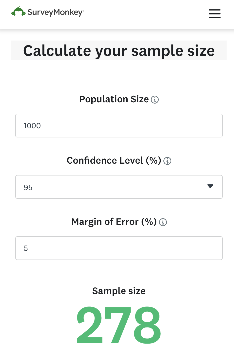
If we calculate a sample size of 385 using the original formula for a large population, but the actual population is 1000 student assignments, the adjusted sample size would be:
$$ n_{adj} = \frac{385}{1 + \frac{385 - 1}{1000}} \approx 278 $$
Thus, if the population size is finite, we would only need to sample 278 assignments instead of 385.
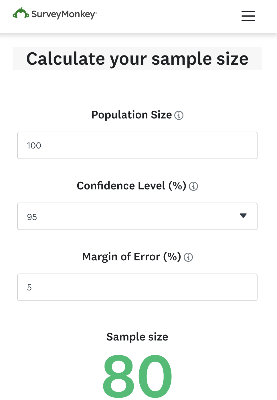
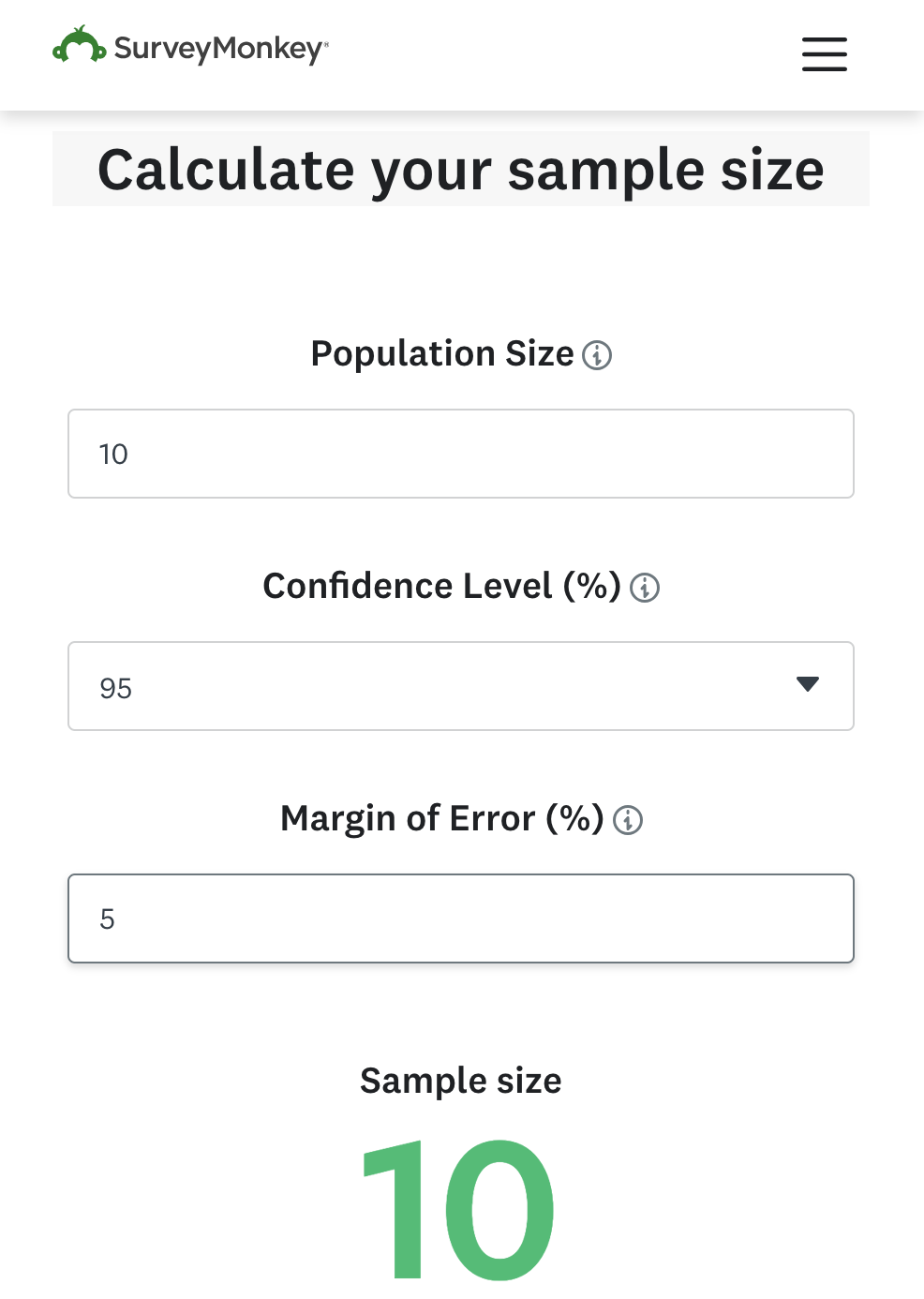
Online sample size calculator
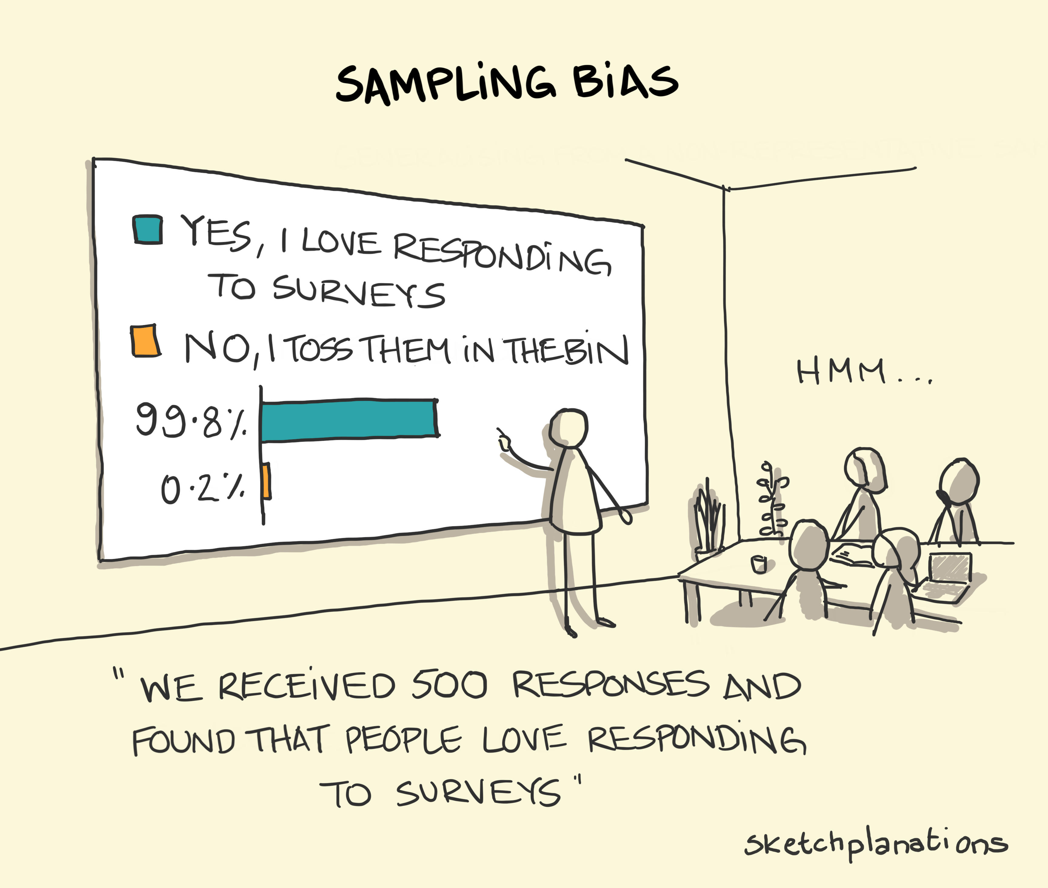
Sampling Bias and Error
Types of Bias:
-
Selection Bias: Occurs when the sample is not representative of the population.
Example: Sampling only high-performing students leads to a biased understanding of overall student performance.
-
Response Bias: Arises when participants respond inaccurately, either intentionally or unintentionally.
Example: Students might not fully complete their assignments, leading to misleading insights.
Minimizing Bias:
- Use Random Sampling Methods: Ensure every student or assignment has an equal chance of being selected.
- Ensure Sample Representation: Account for diversity in assignment types, student abilities, etc.
Avoid sampling only high-performing students to get a representative view.
Selecting each student’s work as a sample:
-
Benefit: Ensures that every student is represented, allowing for an inclusive and complete understanding of overall performance.
Example: By selecting at least one assignment from each student, we capture a broader range of abilities and work styles, and ensure each student’s work contributes to the overall analysis. This is also useful in providing feedback to each student.
-
Risk: The quality of work may vary depending on the assignment. Some students might put more effort into one assignment than another, which may not reflect their overall abilities.
Example: A student might perform exceptionally well on one assignment but poorly on others. Sampling only one assignment could give an incomplete picture of their performance.
How to sample if we have 60 unique students and a required sample size of 278 assignments out of 1000 assignments, if all 60 students need to be represented in the sample
- Determine the number of assignments to sample from each student to ensure that every student is represented. Since we have 60 students, a basic approach is to start by sampling a minimum number of assignments per student.
- Allocate assignments to each student such that all students are included in the sample. For example, start with sampling at least one assignment from each student.
- After ensuring that each student is represented, calculate the remaining number of assignments needed to reach the total sample size of 278.
- Randomly select additional assignments from the students to meet the required sample size. Ensure that the total number of sampled assignments equals 278.