Topics on High-Dimensional Data Analytics
- Introduction
- Functional Data Analysis
- Image Analysis
- Tensor Data Analysis
- Optimization and Application
- Regularization
Introduction
Big Data
Big data is a term used to describe extremely large and complex datasets that traditional data processing applications are not well-equipped to handle. The concept of “big data” is often associated with what is referred to as the “4V” framework, which describes the key characteristics of big data:
- Volume: This refers to the sheer scale of data generated and collected. Big data involves datasets that are too large to be managed and processed using traditional databases and tools. This massive volume can range from terabytes to petabytes and beyond.
- Velocity: This characteristic pertains to the speed at which data is generated, collected, and processed. In today’s fast-paced digital world, data is generated at an unprecedented rate, often in real-time or near-real-time. Examples include social media interactions, sensor data from IoT devices, financial transactions, and more.
- Variety: Big data comes in various formats and types, such as structured, semi-structured, and unstructured data. Structured data is organized into a well-defined format (e.g., tables in a relational database), whereas unstructured data lacks a specific structure (e.g., text documents, images, videos, social media posts). Semi-structured data lies somewhere in between, having a partial structure but not fitting neatly into traditional databases.
- Veracity: Veracity refers to the quality and reliability of the data. With the proliferation of data sources, there’s an increased potential for data to be incomplete, inaccurate, or inconsistent. Ensuring the accuracy and trustworthiness of big data is a significant challenge, and data quality management is crucial for meaningful insights.
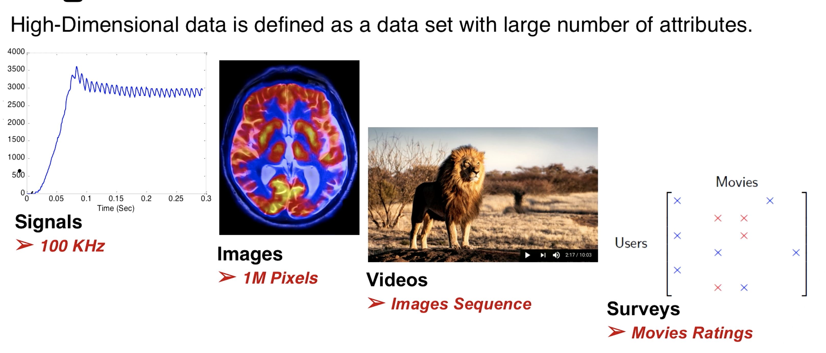
High Dimensional Data
High-dimensional data refers to datasets where the number of features or variables (dimensions) is significantly larger than the number of observations or samples. In other words, the data has a high number of attributes compared to the number of data points available. This kind of data is prevalent in various fields such as genomics, image analysis, social networks, and more.
Difference between High Dimensional Data and Big Data
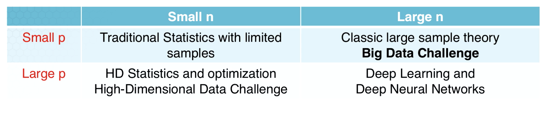
p = dimension n = samples
The Curse of Dimensionality
As the number of features or dimensions grows, the amount of data we need to generalize accurately grows exponentially!
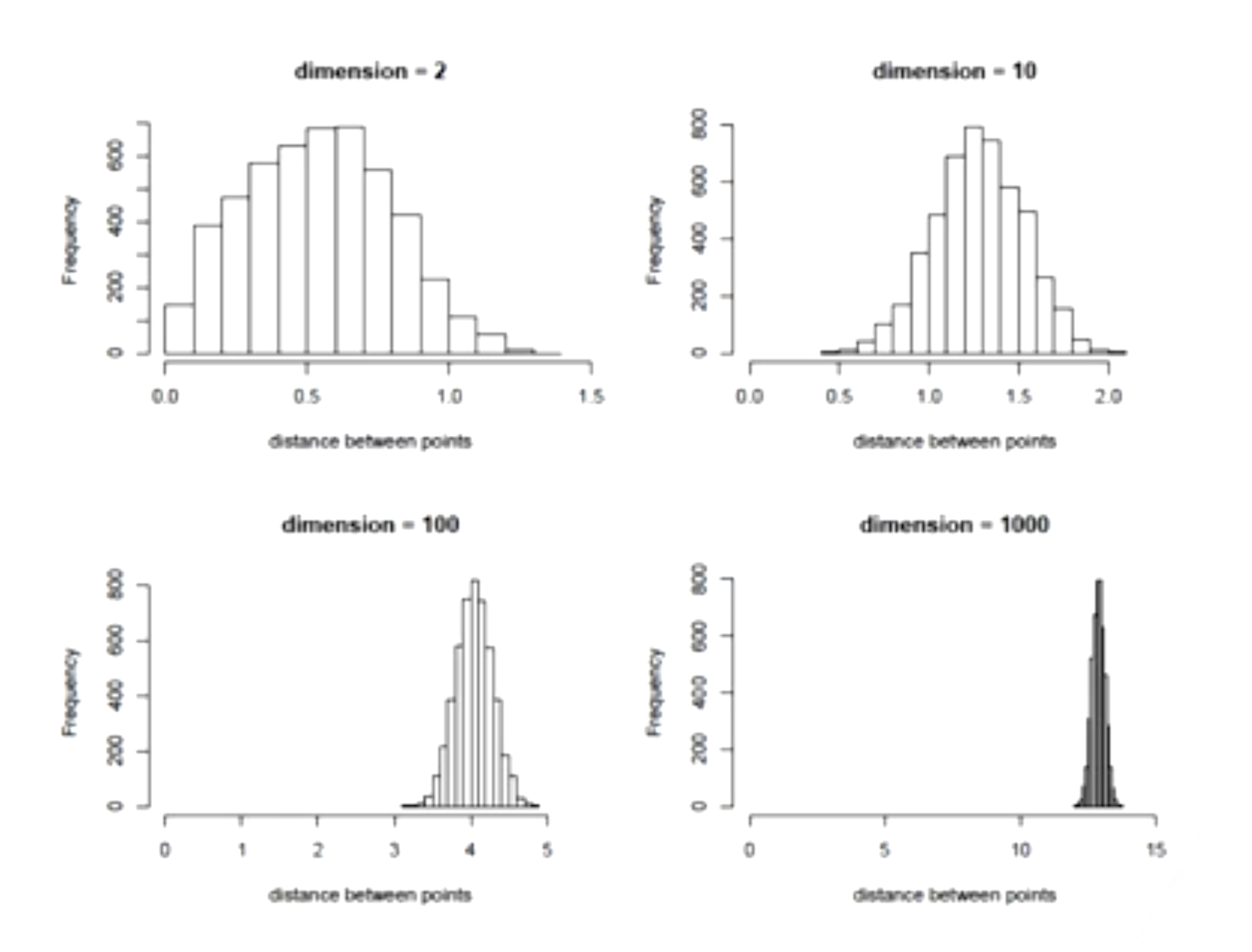
As distance between observations increases with the dimensions, the sample size required for learning a model drastically increases.
- Increased Sparsity: In higher dimensions, the available data points are spread out more thinly across the space. This means that data points become farther apart from each other, making it challenging to find meaningful clusters or patterns. It’s like having a lot of points scattered in a large, high-dimensional space, and they’re so spread out that it’s difficult to identify any consistent relationships.
- More Data Needed: With higher-dimensional data, you need a disproportionately larger amount of data to capture the underlying patterns accurately. When the data is sparse, it’s harder to generalize from the observed points to make accurate predictions or draw conclusions. As the dimensionality increases, you might need exponentially more data to maintain the same level of accuracy in your models.
- Impact on Complexity: The complexity of machine learning models increases with dimensionality. More dimensions mean more parameters to estimate, which can lead to overfitting – a situation where a model fits the training data too closely and fails to generalize well to new data.
- Increased Computational Demands: Processing and analyzing high-dimensional data require more computational resources and time. Many algorithms become slower and more memory-intensive as the number of dimensions grows. This can make experimentation and model training more challenging and time-consuming.
- Difficulties in Visualization: Our ability to visualize data effectively diminishes as the number of dimensions increases. We are accustomed to thinking in 2D and 3D space, but visualizing data in, say, 10 dimensions is practically impossible. This can make it hard to understand the structure of the data and the relationships between variables.
Low Dimensional Learning From High Dimensional Data
High dimensional data usually have low dimensional structure.
This can be achieved through Functional Data Analysis, Tensor Analysis, Rank Deficient Methods among others.
Solutions for the curse of dimensionality
- Feature extraction
- Dimensionality reduction
- Collecting much more observations
Functional Data Analysis
A fluctuating quantity or impulse whose variations represent information and is often represented as a function of time or space.
From Wikipedia
Functional data analysis (FDA) is a branch of statistics that analyses data providing information about curves, surfaces or anything else varying over a continuum. In its most general form, under an FDA framework, each sample element of functional data is considered to be a random function. The physical continuum over which these functions are defined is often time, but may also be spatial location, wavelength, probability, etc. Intrinsically, functional data are infinite dimensional. The high intrinsic dimensionality of these data brings challenges for theory as well as computation, where these challenges vary with how the functional data were sampled. However, the high or infinite dimensional structure of the data is a rich source of information and there are many interesting challenges for research and data analysis.

Regression - Least square Estimates
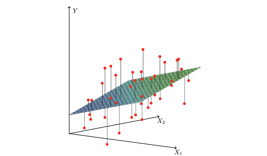
A linear regression model assumes that the regression function $E(Y|X)$ is linear in the inputs $X_1, …, X_p$. They were developed in the pre-computer age of statistics, but even in today’s computer era there are still good reasons to study and use them. They are simple and often provide an adequate and interpretable description of how the inputs affect the output.
The linear regression model has the form:
$f(X) = \beta_0 + \sum_{j=1}^p X_j\beta_j$
Typically we have a set of training data $(x_1, y_1)…(x_N, y_N)$ from which to estimate the parameters $\beta$. Each $x_i = (x_{i1}, x_{i2} … x_{ip})^T$ is a vector of feature measurements for the $i$th case. The most popular estimation method is the least squares, in which we pick the coefficients $\beta = (\beta_0, \beta_1,….\beta_p)^T$ to minimize the residual sum of squares.
$\sum_{i=1}^N (y_i - f(x))^2 = \sum_{i=1}^N (y_i - \beta_0 - \sum_{j=1}^p X_j\beta_j)^2$
Denote $X$ by the $N \times (p+1)$ matrix with each row an input vector (with a 1 in the first position, to represent the intercept), and similarity let $y$ be the $N$ vector of outputs in the training set. Then we can write the residual sum-of-squares as :
$RSS(\beta) = (y-X\beta)^T(y-X\beta)$
Differentiating with respect to $\beta$, ….
$\hat{\beta} = (X^TX)^{-1}X^Ty$
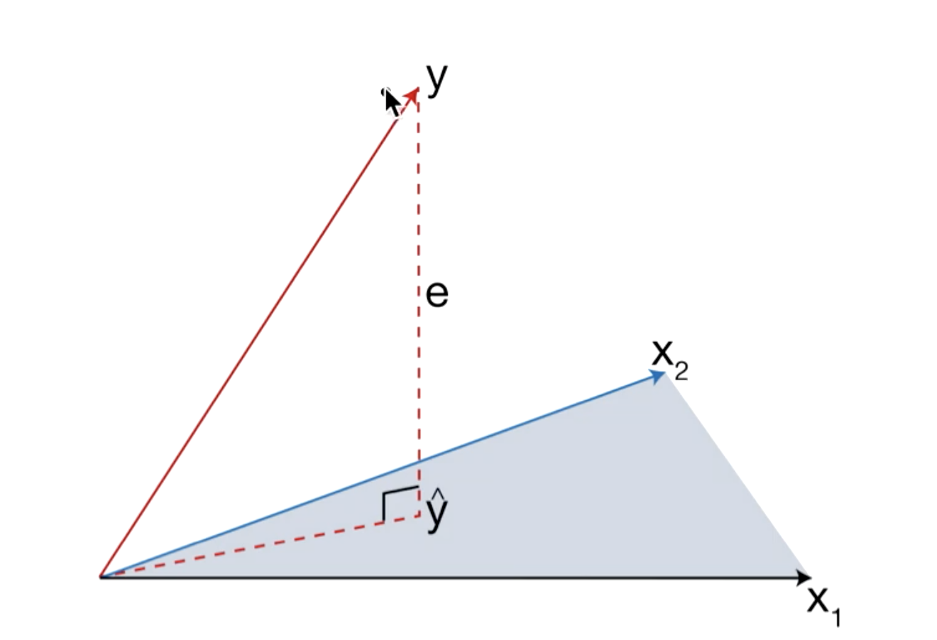
Geometric Interpretation
$\hat{y} = X\hat{\beta} = X(X^TX)^{-1}X^Ty = Hy $
Projection Matrix (or Hat matrix): The outcome vector $y$ is orthogonally projected onto the hyperplane spanned by the input vectors $x_1$ and $x_2$. The Projection $\hat{y}$ represents the vector of predictions obtained by the least square method.
Properties of OLS
- They are unbiased estimators. That is the expected value of estimators and actual parameters are the same $E(\hat{\beta}) = \beta$
- The covariance can be obtained by $cov(\hat{\beta}) = \sigma^2 (X^TX)^{-1}$, where $\sigma^2 = SSE/(n-p)$
- According to the Gauss-Markov Theorem, among all unbiased linear estimates, the least square estimate (LSE) has the minimum variance and it is unique.
Regression can be used for Feature Extraction
Splines
Polynomial Regression is a type of regression analysis where the relationship between the independent variable (input) and the dependent variable (output) is modeled as an nth-degree polynomial. In other words, instead of fitting a straight line (linear regression), a polynomial regression can fit curves of various degrees, allowing for more flexibility in capturing complex relationships. For example, a quadratic polynomial regression (degree 2) can model a parabolic relationship, and a cubic polynomial regression (degree 3) can model more intricate curves.
Polynomial regression is still considered a type of linear regression because the relationship between the input and output variables is linear with respect to the coefficients, even though the input variables may be raised to different powers. The model equation for polynomial regression of degree n is:
$y = \beta_0 + \beta_1x + \beta_2x^2 + \beta_3x^3 + … + \beta_mx^m + \epsilon$
Nonlinear Regression, on the other hand, refers to a broader class of regression models where the relationship between the independent and dependent variables is not a linear function. Nonlinear regression can encompass a wide range of functional forms, including exponential, logarithmic, sigmoidal, and other complex shapes. The main characteristic of nonlinear regression is that the model parameters are estimated in a way that best fits the chosen nonlinear function to the data.
Unlike polynomial regression, nonlinear regression models can’t be expressed in terms of a simple equation with polynomial terms. The specific form of the nonlinear function needs to be determined based on the problem’s nature and domain knowledge.
Disadvantages of Polynomial Regression
- Remote part of the function is very sensitive to outliers
- Less flexibility due to global function structure
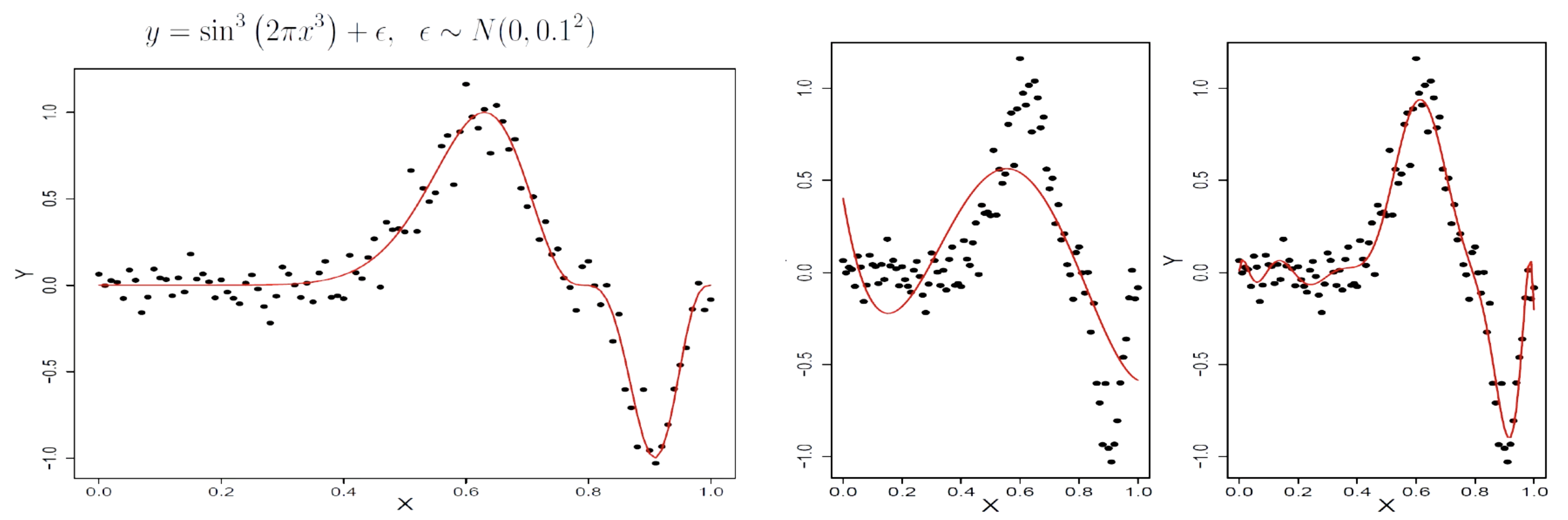
The global function structure causes underfitting or overfitting.
The solution is to move from global to local structure -> Splines.
Splines
- Linear combination of Piecewise Polynomial Function under continuity assumption
- Partition the domain of x into continuous intervals and fit polynomials in each interval separately
- Provides flexibility and local fitting
Suppose $x \in [a,b]$. Partition the x domain using the following points (a.k.a knots):
$a<\xi_1<\xi_2…<\xi_k<b, <\xi_0=a, <\xi_{k+1}=b$
Fit a polynomial in each interval under the continuity conditions and integrate them by
$f(X) = \sum_{m=1}^K \beta_mh_m(X)$
Simple Example
Piecewise Constant
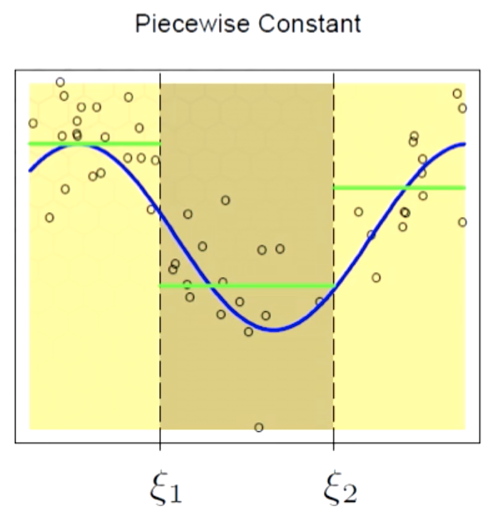
Here we are using a zero order polynomial. A zero order polynomial can be defined by an indicator function. If we use OLS, the beta would be the average of point in each local region.
$f(X) = \sum_{m=1}^3 \beta_mh_m(X)$
Piecewise Linear
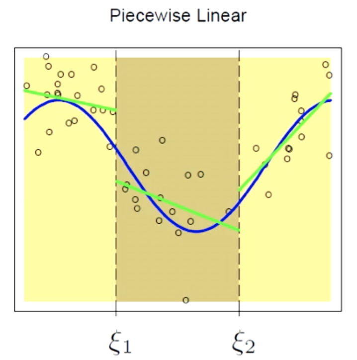
Here we are using a first order polynomial. A first order polynomial includes slopes and intercept (and therefore $K=6$ here.)
$f(X) = \sum_{m=1}^6 \beta_mh_m(X)$
There are two issues here:
- Discontinuity
- Underfitting
Solving for Discontinuity
We can impose continuity constraint for each knot:
$f{\xi^-_1}=f(\xi^+_1)$
This can be translated to $\beta_1+\xi_1\beta_4 = \beta_2 + \xi_1\beta_5$
Not sure how
By adding constraints we are losing some degrees of freedom. The total number of free parameters (degree of freedom) = 6 (total number of parameters -2 (total number of constraints) = 4
Alternatively, once could incorporate the constraints into the basis functions:
$h_1(X) = 1$,
$h_2(X) = X$,
$h_3(X) = (X-\xi_1)_+$,
$h_4(X) = (X-\xi_2)_+$
This basis is known as truncated power basis
$(X-\xi_k)_+ = (X-\xi_k)$ if $x \ge xi_k$ $0$ if $x<xi_k$
Solving for Underfitting
Splines with Higher Order of Continuity can be used to tackle underfitting.
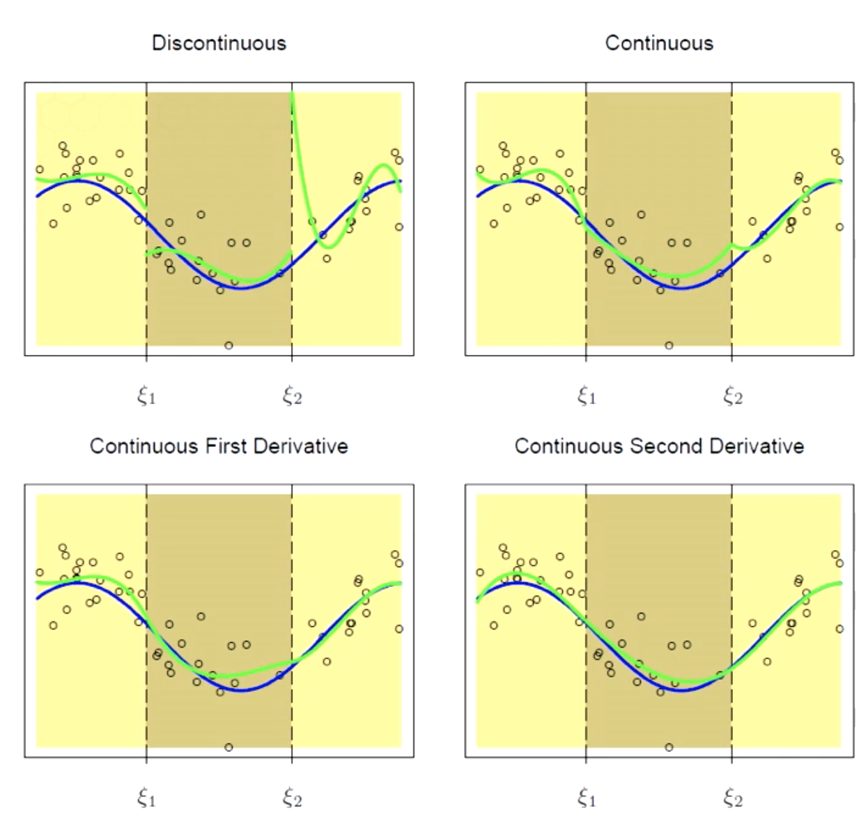
Continuity constraints for smoothness
$f{\xi^-_1}=f(\xi^+_1)$
$f^’{\xi^-_1}=f^’(\xi^+_1)$
$f^{’’}{\xi^-_1}=f^{’’}(\xi^+_1)$
$h_1(X) = 1$,
$h_2(X) = X$,
$h_3(X) = X^2$,
$h_4(X) = X^3$,
$h_5(X) = (X-\xi_1)^3_+$,
$h_6(X) = (X-\xi_2)^3_+$
The degree of freedom is calculated by: Number of regions * Number of parameters in each region) - (Number of knots)*(Number of constraints per knot)
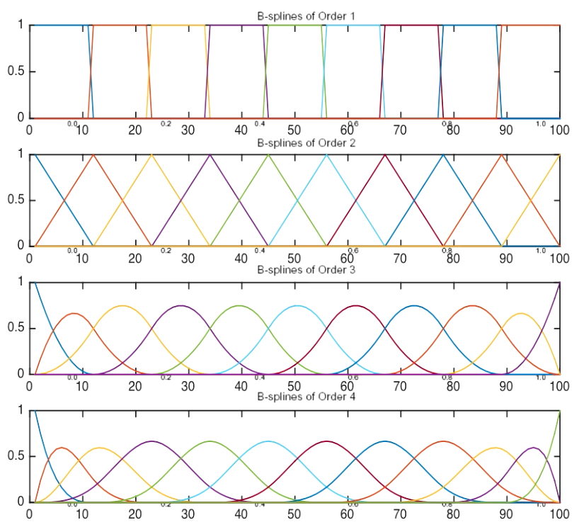
Order-M Splines
- M=1 piecewise-constant splines
- M=2 linear splines
- M=3 quadratic splines
- M=4 cubic splines
For Truncated power basis functions:
- Total degree of freedom is K+M
- Cubic spline is the lowest order spline for which the knot discontinuity is not visible to human eyes
- Knots selection: a simple method is to use x quantiles. However, the choice of knots is a variable/model selection problem.
Estimation
- After creating the basis function, we can use OLS to estimate parameters $\beta$
- First of all, create a basis matrix by concatinating basis vectors. For example if we have cubic splines with two knots, we will have six basis vectors.
$H = [h_1(x) \quad h_2(x) \quad h_3(x) \quad h_4(x) \quad h_5(x) \quad h_6(x)]$
gives $\hat\beta = (H^TH)^-1H^Ty$
Linear Smoother: $\hat y= H\hat\beta = H(H^TH)^{-1}H^Ty = Sy$
Degrees of Freedom $df=trace S$
Although truncated power basis functions are simple and algebraically appealing, it is not efficient for computation and ill-posed and numerically unstable. The matrix is close to singular (because of correlations among themselves, and determinant being very close to zero), and inverting it becomes challenging.
The solution is to user Bsplines.
Bsplines
- Alternative basis vectors for piecewise polynomials that are computationally more efficient
- Each basis function has a local support, that is, it is nonzero over at most M (spline order) consecutive intervals
- The basis matrix is banded
- The low bandwidth of the matrix reduces the linear dependency of the columns, and therefore, removes the numeric column stability.
Bspline Basis
Let $B_{j,m}(x)$ be the $j^{th}$ B-spline basis function of order $m(m \le M)$ for the knot sequence $\tau$
$a < \xi_1 < \xi_2 < … < \xi_k < b$
Define the augmented knots sequence $\tau$
$\tau_1 \le \tau_2 …\le \tau_M \le \xi_0$ (before the lower bound)
$\tau_{M+j} = \xi_j, j = 1, … , K$
$\xi_{K+1} \le \tau_{M+K+1} \le \tau_{M+K+2} \le … \le \tau_{2M+K}$ (after the lower bound)
Smoother Matrix
Consider a regression Spline basis B
$\hat f = B(B^TB)^{-1}B^Ty = Hy$
- H is the smoother matrix (projection matrix)
- H is idempotent ($H \times H = H$)
- H is symmetric
- Degrees of freedom trace (H)
Smoothing Splines
Bspline basis boundary issue
Consider the following setting with the fixed training data
$y_i = f(x_i) + \epsilon_i$
$\epsilon_i \approx iid(0, \sigma^2)$
$Var(\hat f(x)) = h(x)^T(H^TH)^{-1}h(x)\sigma^2$ (variance of estimated function using spline)
Behavior of splines tends to be sporadic near the boundaries, and extrapolation can be problematic. The main reason is that the complexity of Cubic Spline is more than the complexity of Global Cubic Polynomial, due to the large number of parameters (less bias, more variance). The solution is to use linear splines instead of cubic splines (Natural Cubic Splines).
Natural Cubic Splines
- Additional constraints are added to make the function linear beyond the boundary knots
- Assuming the function is linear near the boundaries (where there is less information) is often reasonable
- Cubic spline; linear on $[-\inf, \xi_1]$ and $[\xi_k , \inf]$
- Prediction variance decreases
- The price is the bias near the boundaries
- Degrees of freedom is K, the number of knots
- Each of these basis functions has zero second and third derivative in the linear region.
Penalized residual sum of squares
$\min_f \frac{1}{n}\sum_{i-1}^n[y_i - f(x_i)]^2+\lambda \int^a_b[f^{"}(x)^2dx]$
- The first term measures the closeness of the model to the data (related to bias)
- The second term penalizes curvature of the function (related to variance)
- $\lambda$ is the smoothing parameter controlling the trade between bias and variance
- $\lambda = 0$ interpolate the data (overfitting)
- $\lambda = \inf$ linear least-square regression (underfitting)
It can be shown that the minimizer is a natural cubic spline.
Solution: $\hat \theta = (N^TN + \lambda\Omega)^{-1}N^Ty$ , $\Omega$ represents the second derivative
$ f = (N^TN + \lambda\Omega)^{-1}N^Ty = S_\lambda y$
- Smoothing spline estimator is a linear smoother
- $S_\lambda$ is the smoother matrix
- $S_\lambda$ is NOT idempotent
- $S_\lambda$ is symmetric
- $S_\lambda$ is positive definite
- Degrees of freedom: trace($S_\lambda$)
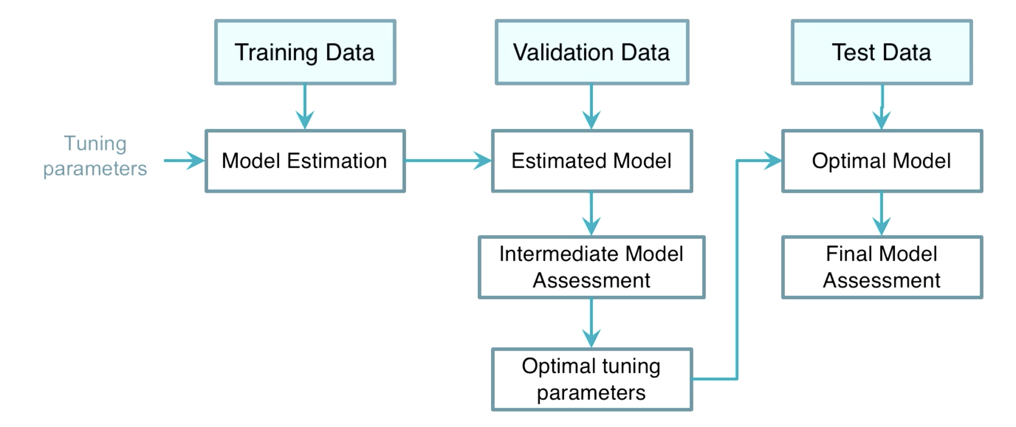
Choice of Tuning Parameters
-
Train Test Validation
-
Cross Validation If an independent validation dataset is not affordable, the K-fold cross validation or leave-one-out CV can be useful
-
Akaike Information Criteria (AIC)
-
Bayesian Information Criteria (BIC)
-
Generalized Cross-validation
Kernel Smoothers
K-Nearest Neighbor (KNN)
KNN Average $\hat f(x_0) = \sum_{i=1}^nw(x_0, x_i)y_i$
where $\sum_{i=1}^nw(x_0, x_i)$ = $\frac{1}{K}$ if $x_i \in N_k(x_0)$ else $0$
- Simple average of the k nearest observations to $x_0$ (local averaging)
- Equal weights are assigned to all neighbors
- However, the fitted function is in the form of a step function (non-smooth function)
- Also, the bias is quite high
Kernel Function
Any non-negative real-valued integrable function that satisfies the following conditions:
- $\int_{-\inf}^{\inf}K(u)du=1$
- K is an even function; $K(-u) = K(u)$
- It has a finite second moment; $u^2\int_{-\inf}^{\inf}K(u)du < \inf$
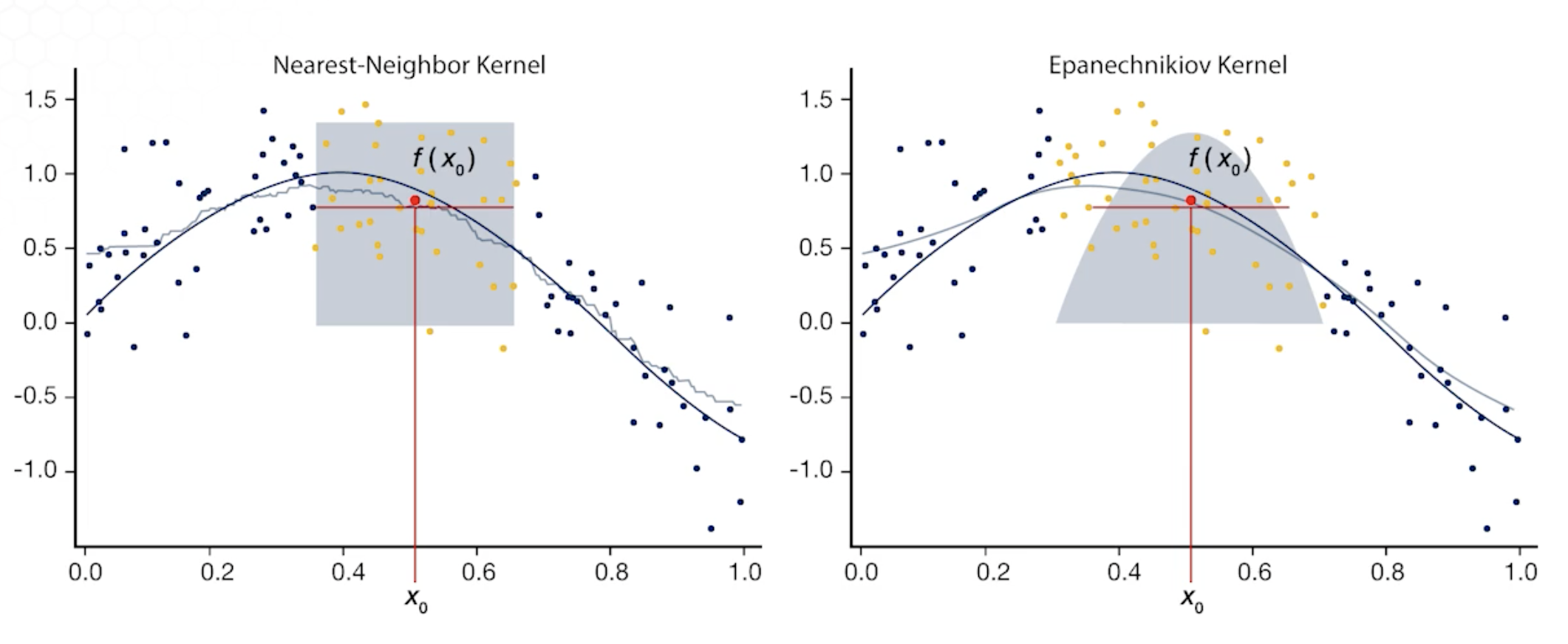
Kernel Smoother Regression
Kernel Regression
- Is weighted local averaging that fits a simple model separately at each query point $x_0$
- More weights are assigned to closer observation
- Localization is defined by the weighting function
- Kernel regression requires little training, all calculations get done at the evaluation time.
Choice of $\lambda$
- $\lambda$ defines the width of the neighbourhood
- Only points withing $[x_0-\lambda, x_0+\lambda]$ receive positive weights
- Smaller $\lambda$: rough estimate, larger bias, smaller variance
- Larger $\lambda$: smoother estimate, smaller bias, larger variance
Cross-validation can be used for determining of $\lambda$:
Drawbacks of Local Averaging
- The local averaging can be biased on the boundaries of the domain due to the asymmetry of the kernel in that region.
- This can be solved by local linear regression
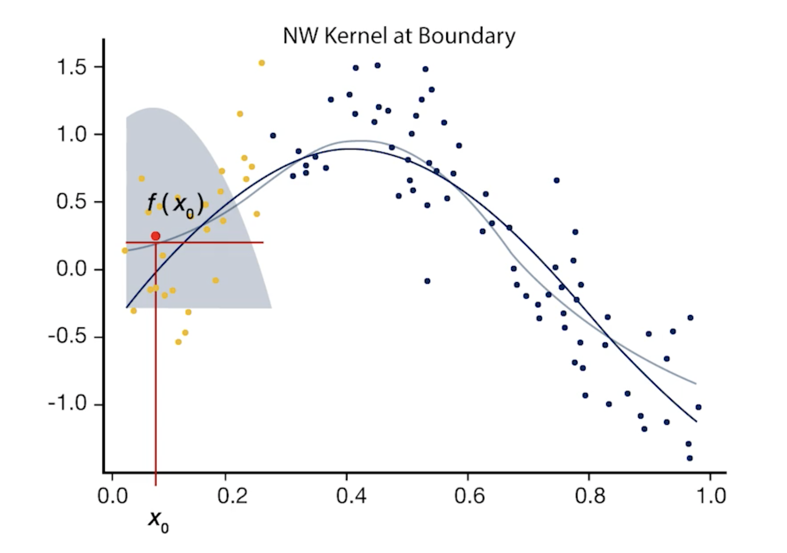
- Local linear regression corrects the bias on the boundaries
- Local polynomial regression corrects the bias in the curvature region
- However, local polynomial regression is complex due to higher order of polynomials, therefore, it increases the prediction variance.
- A good solution would be to use local linear model for points in the boundaries, and local quadratic regression in the interior regions.
Functional Principal Component
Similar to PCA, FPCA aims to reduce the dimension of functional data by extracting a small set of uncorrelated features, which capture the most of the variation.
Functional data (observed signals) are comprised of two main components. The first component is the continuous functional mean, and the second component is the error term, that is, the realizations from a stochastic process with mean function 0 and covariance function $C(t, t^’)$. It includes both random noise and signal-to-signal variations
$s_i(t) = \mu(t) + \epsilon_i(t)$
The mean function is common across all signals (notice that it does not have the $i$ subscript)
Since signal variance comes from the noise function, we first focus on this for dimensionality reduction using the Karhunen-Loeve Theorem.
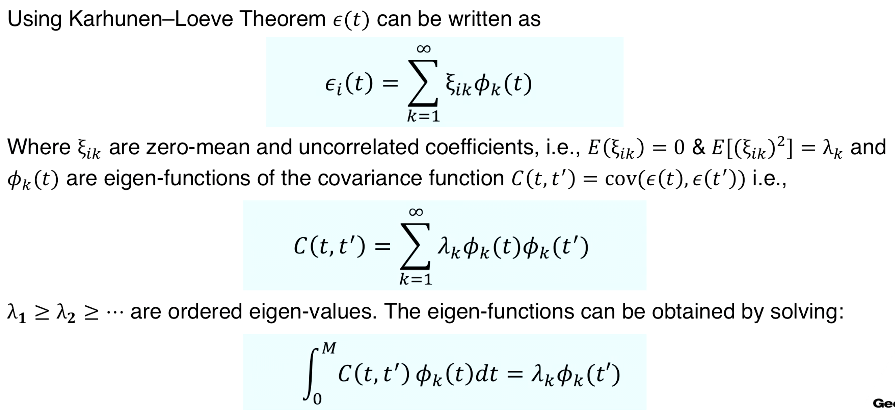
The variance of $\xi_{ik}$ quickly decays with k. Therefore, only a few $\xi_{ik}$ also known as FPC-scores, would be enough to accurately approximate the noise function. That is,
$\epsilon_i(t) \approx \sum_{k=1}^K \xi_{ik}\phi_{k}(t)$
Signals decomposition is given by
$s_i(t) = \mu(t) + \epsilon_i(t) \implies \mu(t) + \sum_{k=1}^K \xi_{ik}\phi_{k}(t)$
Model Estimation
Both the mean and covariance is unknown, and should be measured using training data. In practice, we have two types of signals/data:
- Complete signals: Sampled regularly
- Incomplete signals: Sampled irregularly, sparse, fragmented
Steps for FPCA when the signals are incomplete:
- Estimate the mean function using local linear regression
- Estimate the raw covariance function using the estimated mean function
- Estimate the covariance surface using local quadratic regression
- Compute the Eigen functions
- Compute the FPC scores
Image Analysis
Introduction to Image Processing
- The process of processing raw images and extracting useful information for decision making.
- Level 0: Image representation (acquisition, sampling, quantization, compression)
- Level 1: Image to Image transformations (enhancement, filtering, restoration, smoothing, segmentation)
- Level 2: Image to vector transformation (feature extraction and dimension reduction)
- Level 3: Feature to decision mapping
What is an Image?
A gray (color-RGB) image is a 2-D (3-D) light intensity function, $f (x_1, x_2)$, where $f$ measures brightness at position $f(x_1, x_2)$ . A digital gray (color) image is a representation of an image by a 2-D (3-D) array of discrete samples. Pixel is referred to an element of the array.
Possible values each pixel can have:
- Black and white image: 2
- 8-bit Gray image: 256
- RGB: 256 x 256 x 256 = 16777216
Basic Manipulation in Python
import cv2

# Load the image
image_path = 'your_image.jpg'  # Replace with the path to your image
original_image = cv2.imread(image_path)

# Check if the image was loaded successfully
if original_image is None:
    print("Error: Could not open or find the image.")
else:
    # Convert the image to grayscale
    gray_image = cv2.cvtColor(original_image, cv2.COLOR_BGR2GRAY)

    # Convert the grayscale image to black and white using thresholding
    _, binary_image = cv2.threshold(gray_image, 128, 255, cv2.THRESH_BINARY)

    # Resize the image (e.g., to a width of 800 pixels while maintaining aspect ratio)
    new_width = 800
    aspect_ratio = original_image.shape[1] / original_image.shape[0]
    new_height = int(new_width / aspect_ratio)
    resized_image = cv2.resize(binary_image, (new_width, new_height))

    # Save the processed images to disk
    cv2.imwrite('gray_image.jpg', gray_image)
    cv2.imwrite('black_and_white_image.jpg', binary_image)
    cv2.imwrite('resized_image.jpg', resized_image)

    print("Images processed and saved successfully.")
Image Transformation
Image Histogram
- Histogram represents the distribution of gray levels.
- It is an estimate of the probability density function (pdf) of the underlying random process.
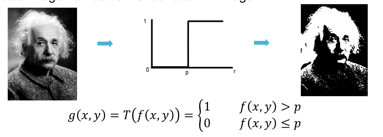
Image can be transformed by applying a function on the image matrix.
$g(x,y) = T(f(x,y))$
For example if a threshold function is sued as the transformation function a gray-scale image can be converted to a BW image.
- The brightness of an image can be changed by shifting its histogram.
- The contrast of an image is defined by the difference in maximum and minimum pixel intensity.
- Gray level resolution refers to change in the shades or levels of gray in an image.
- The number of different colors in an image depends on bits per pixel (bpp).
$L = 2^{bpp}$
- Gray level transformation is often used for image enchantment.
- Three typical transformation functions are:
- Linear (negative image)
- Log
- Power-Law
Convolution and image filtering
The convolution of functions $f$ and $g$ is defined by:
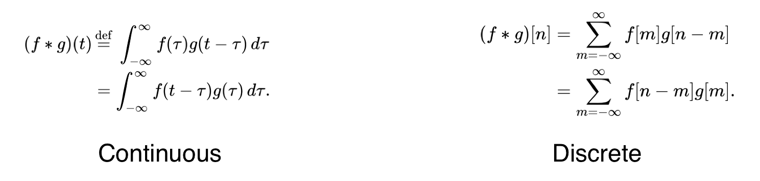
- Convolution is widely used in image processing for denoising, blurring, sharpening, embossing, and edge detection.
- Image filter is a convolution of a mask (aka kernel, and convolution matrix) with an image that can be used for blurring, sharpening, edge detection, etc.
- A mask is a matrix convolved with an image.
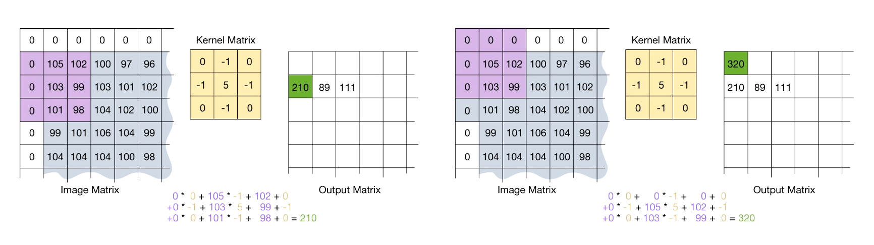
Image Convolution with a Mask
- Flip the mask (kernel) both horizontally and vertically.
- Put the center element of the mask at every pixel of the image. Multiply the corresponding elements and then add them up. Replace the pixel value corresponding to the center of the mask with the resulting sum.
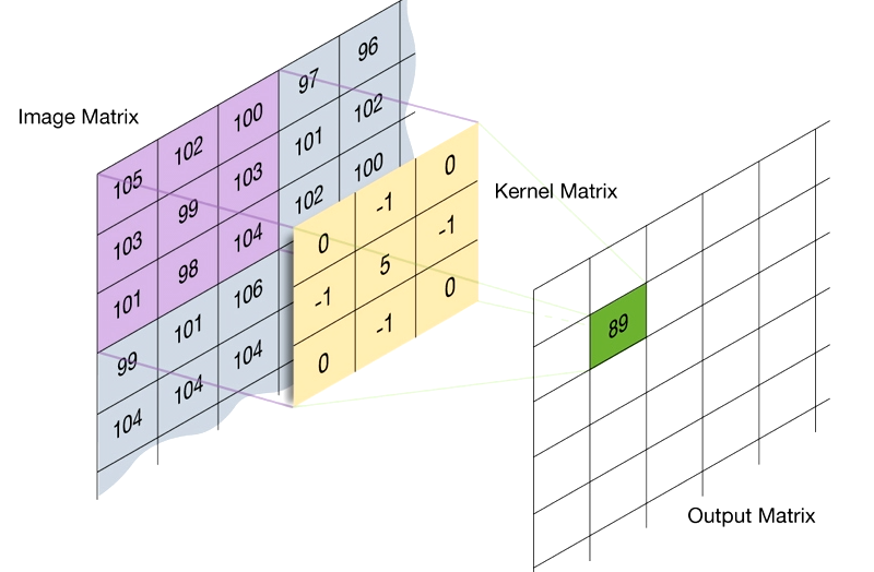
- For pixels on the border of image matrix, some elements of the mask might fall out of the image matrix. In this case, we can extend the image by adding zeros. This is known as padding.
Denoising of Smooth Images using Splines
- Another approach for denoising smooth images is to use local regression with smooth basis (eg. splines)
- Using Kronecker product, a 2D-spline basis can be generated from 1D basis matrices
Image Segmentation
- The main goal of image segmentation is to partition an image into multiple sets of pixels (segments)
- Image segmentation has been widely used for object detection, face and fingerprint recognition, medical imaging, video surveillance, etc.
- Various methods exist for image segmentation including:
- Local and global thresholding
- Otsu’s method
- K-means clustering
- Thresholding is a simple segmentation approach that converts grayscale image to binary image by applying the thresholding function on histogram.
Otsu’s Method
- The goal is to automatically determine the threshold $t$ given an image histogram.
Steps:
- Get the histogram of the image
- Calculate group mean and variance
- Find the maximum value for the variance
- Threshold the image
import numpy as np

def compute_otsu_criteria(im, th):
    """Otsu's method to compute criteria."""
    # create the thresholded image
    thresholded_im = np.zeros(im.shape)
    thresholded_im[im >= th] = 1

    # compute weights
    nb_pixels = im.size
    nb_pixels1 = np.count_nonzero(thresholded_im)
    weight1 = nb_pixels1 / nb_pixels
    weight0 = 1 - weight1

    # if one of the classes is empty, eg all pixels are below or above the threshold, that threshold will not be considered
    # in the search for the best threshold
    if weight1 == 0 or weight0 == 0:
        return np.inf

    # find all pixels belonging to each class
    val_pixels1 = im[thresholded_im == 1]
    val_pixels0 = im[thresholded_im == 0]

    # compute variance of these classes
    var1 = np.var(val_pixels1) if len(val_pixels1) > 0 else 0
    var0 = np.var(val_pixels0) if len(val_pixels0) > 0 else 0

    return weight0 * var0 + weight1 * var1

im = # load your image as a numpy array.
# For testing purposes, one can use for example im = np.random.randint(0,255, size = (50,50))

# testing all thresholds from 0 to the maximum of the image
threshold_range = range(np.max(im)+1)
criterias = [compute_otsu_criteria(im, th) for th in threshold_range]

# best threshold is the one minimizing the Otsu criteria
best_threshold = threshold_range[np.argmin(criterias)]
K-Means Clustering Method
K-means clustering is a method for partitioning a set of observations to K clusters, such that the within-cluster variation is minimized.
- Rearrange the image pixels such that the number of rows in the resulting matrix is equal to the number of pixels and the number of columns is the same as the number of color channels
- Randomly select K centers
- Assign each pixel to the closest cluster
- Update the cluster mean
- Repeat the last two process until convergence
The objective of K-means is to minimize the within cluster variation, and maximize the inter-class variation.
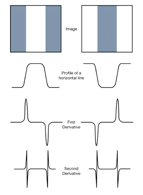
Edge Detection
- Edges are significant local changes of intensity in an image.
- Edge Detection: Detect pixel with sudden intensity change
- Often points that lie on an edge are detected by:
- Detecting the local maxima or minima of the first derivative.
- Detecting the zero-crossings of the second derivative.
Sobel Operator
The Sobel operator works by convolving an image with a pair of 3x3 kernels or filters, one for detecting edges in the horizontal direction (often referred to as the Sobel-X operator) and the other for detecting edges in the vertical direction (often referred to as the Sobel-Y operator). These kernels are as follows:
Sobel-X Kernel:
-1  0  1
-2  0  2
-1  0  1
Sobel-Y Kernel:
-1 -2 -1
 0  0  0
 1  2  1
Krisch Operator
Krisch is another derivative mask that finds the maximum edge strength in eight directions of a compass.
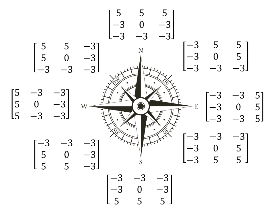
It is more time consuming compare to Sobel
Prewitt Mask
The Prewitt operator, like the Sobel operator, employs a pair of 3x3 convolution kernels, one for detecting edges in the horizontal direction and the other for detecting edges in the vertical direction.
Here are the two Prewitt kernels:
Prewitt-X Kernel:
-1  0  1
-1  0  1
-1  0  1
Prewitt-Y Kernel:
-1 -1 -1
 0  0  0
 1  1  1
Laplacian and Laplacian of Gaussian Mask
- Laplacian mask is a second order derivative mask.
- For noisy images, is combined with a Gaussian mask to reduce the noise
0  1  0
1 -4  1
0  1  0
Laplacian, Sobel, and Prewitt are masks used for edge detection. Gaussian is not a mask for edge detection.
Tensor Data Analysis
Tensor Introduction
A tensor is an algebraic object that describes a multi-linear relationship between sets of algebraic objects related to a vector space. Tensors may map between different objects such as vectors, scalars, and even other tensors.
Terminologies:
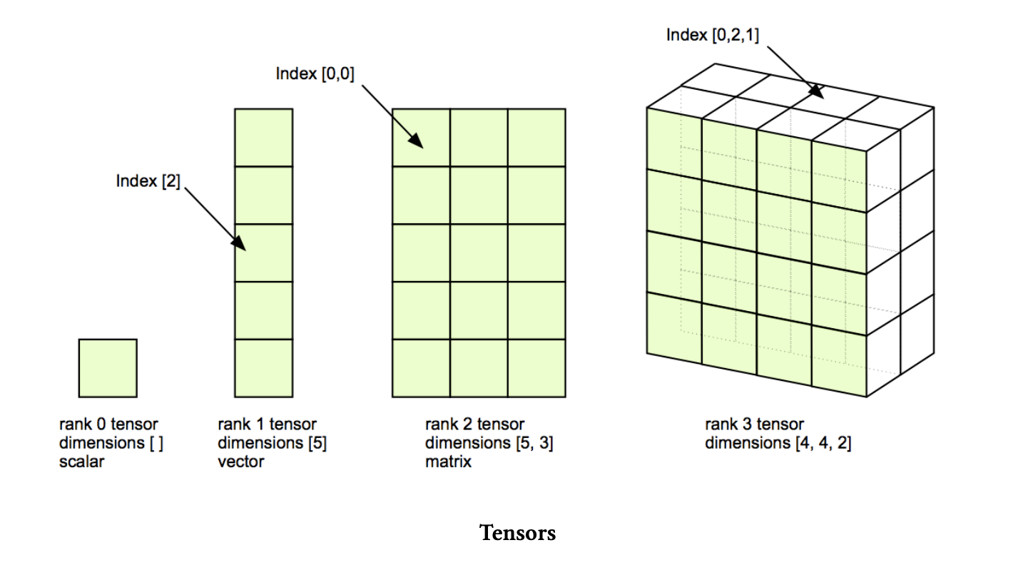
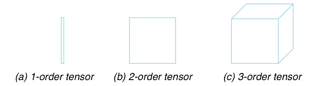
Order
The order of a tensor refers to the number of indices or subscripts needed to specify its components in a given coordinate system. Tensors can have different orders, and the order determines their mathematical properties and how they transform under coordinate transformations. Here’s a brief overview of tensor orders:
Zeroth-Order Tensor (Scalar): A zeroth-order tensor is also known as a scalar. It has no indices and represents a single numerical value. Scalars are invariant under coordinate transformations.
Example: Temperature at a point in space.
First-Order Tensor (Vector): A first-order tensor, also known as a vector, has one index. Vectors represent quantities with both magnitude and direction and transform linearly under coordinate transformations.
Example: Velocity, force, displacement.
Second-Order Tensor (Matrix): A second-order tensor has two indices. It represents a linear transformation that maps one vector to another. Matrices are used to represent various physical quantities, such as stress tensors, moment of inertia tensors, and more.
Example: Stress tensor, moment of inertia tensor.
Third-Order Tensor: A third-order tensor has three indices, and it is used to represent more complex relationships between vectors and matrices. These tensors are less common but can arise in various physical and mathematical contexts.
Example: Piezoelectric tensor in materials science.
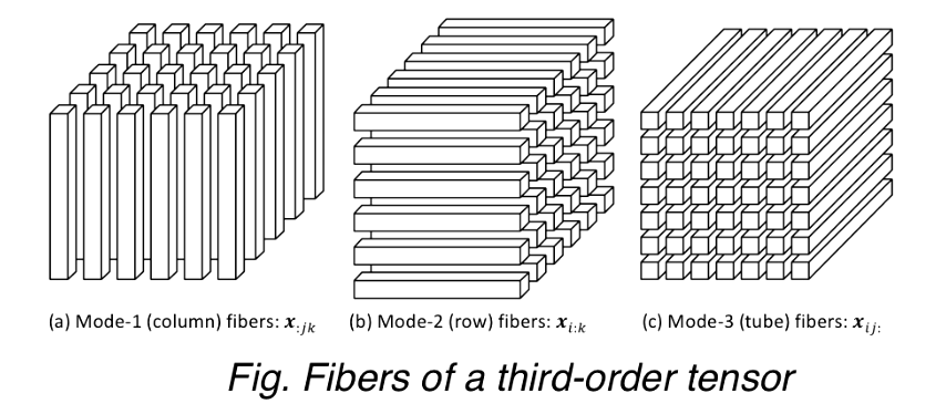
Fibers
A fiber, the higher order analogue of matrix row and column, is defined by fixing every index but one, e.g.,
- A matrix column is a mode-1 fiber and a matrix row is a mode-2 fiber
- Third-order tensors have column, row, and tube fibers
- Extracted fibers from a tensor are assumed to be oriented as column vectors.
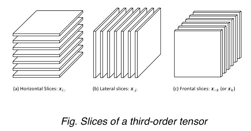
Slices
Two-dimensional sections of a tensor, defined by fixing all but two indices.
Norm
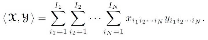
Norm of a tensor $X \in \R^{I_1 \times I_2 \times …. \times I_N}$ is the square root of the sum of the squares of all its elements.
This is analogous to the matrix Frobenius norm, which is denoted $||A||_F$ for matrix $A$
Outer Product
A multi-way vector outer product is a tensor where each element is the product of corresponding elements in vectors
Inner Product
The inner product of two tensors is a generalization of the dot product operation for vectors as calculated by dot. A dot product operation (multiply and sum) is performed on all corresponding dimensions in the tensors, so the operation returns a scalar value. For this operation, the tensors must have the same size.
Using Tensorly for inner and outer product
import tensorly as tl
import numpy as np

# Define the shape of the random tensors
shape = (4, 2, 3)

# Generate random data for X and Y using NumPy
X_data = np.random.rand(*shape)
Y_data = np.random.rand(*shape)

# Convert the NumPy arrays to TensorLy tensors
X = tl.tensor(X_data)
Y = tl.tensor(Y_data)

# Calculate the inner product of X and Y
inner_product = tl.tenalg.inner(X, Y)

# Calculate the outer product of X and Y
outer_product = tl.tenalg.outer(X, Y)

# Print the results
print("Inner Product:")
print(inner_product)

print("\nOuter Product:")
print(outer_product)
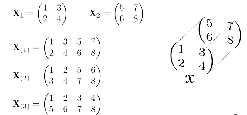
Using Tensorly for unfolding, and flattening
Unfold an N-way tensor into a matrix
import tensorly as tl
import numpy as np

# Create a random 2x2x2 tensor
random_data = np.random.rand(2, 2, 2)
tensor = tl.tensor(random_data)

# Mode-1 matricization (unfold along the first mode)
mode1_matricization = tl.unfold(tensor, mode=0)

# Mode-2 matricization (unfold along the second mode)
mode2_matricization = tl.unfold(tensor, mode=1)

# Mode-3 matricization (unfold along the third mode)
mode3_matricization = tl.unfold(tensor, mode=2)

# Print the results
print("Mode-1 Matricization:")
print(mode1_matricization)

print("\nMode-2 Matricization:")
print(mode2_matricization)

print("\nMode-3 Matricization:")
print(mode3_matricization)
Tensor Multiplication
The n-mode product is referred to as multiplying a tensor by a matrix (or a vector) in mode n.
The n-mode (matrix) product of a tensor $X \in \R^{I_1 \times I_2 \times …. \times I_N}$ with a matrix $U \in R^{J \times I_n}$ is denoted by $X \times_n U$ and is of size $I_1 \times I_2 \times …. \times I_{n-1} \times J \times I_{n+1} \times …\times I_N $
import tensorly as tl
import numpy as np

# Create a random 3x2x4 tensor
random_tensor_data = np.random.rand(3, 2, 4)
tensor = tl.tensor(random_tensor_data)

# Create a random matrix compatible with mode-1 multiplication
random_matrix_data = np.random.rand(2, 5)
matrix = tl.tensor(random_matrix_data)

# Multiply the tensor and matrix in mode-1
result = tl.tenalg.mode_dot(tensor, matrix, mode=1)

# Print the result
print("Random Tensor:")
print(tensor)

print("\nRandom Matrix:")
print(matrix)

print("\nResult of Mode-1 Multiplication:")
print(result)
n-Mode Vector Product
import tensorly as tl
import numpy as np

# Create a random 3x2x4 tensor
random_tensor_data = np.random.rand(3, 2, 4)
tensor = tl.tensor(random_tensor_data)

# Create a random vector compatible with mode-1 multiplication
random_vector_data = np.random.rand(2)
vector = tl.tensor(random_vector_data)

# Multiply the tensor and vector in mode-1
result = tl.tenalg.mode_dot(tensor, vector, mode=1)

# Print the random tensor, random vector, and the result of Mode-1 multiplication
print("Random Tensor:")
print(tensor)

print("\nRandom Vector:")
print(vector)

print("\nResult of Mode-1 Multiplication:")
print(result)
Kronecker Product
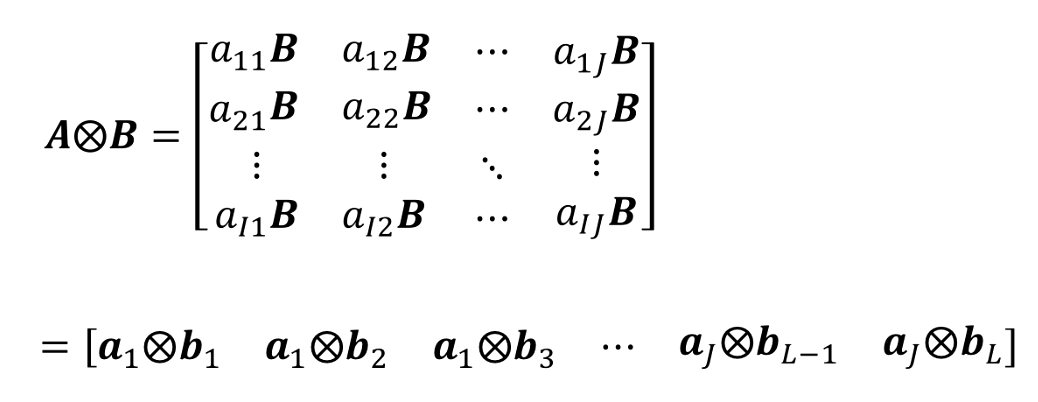
The Kronecker product, denoted by ⊗, is a mathematical operation that combines two matrices to create a larger matrix. It is a tensor product of two matrices and results in a block matrix where each block is a scalar multiple of one of the elements of the first matrix, multiplied by the second matrix.
The Kronecker Product of matrices $A \in R^{I \times J}$ and $B \in R^{K \times L}$ is denoted by $A \bigotimes B$. The result is a matrix size ($IK) \times (JL)$ and defined by
Examples


import numpy as np

# Create two matrices
A = np.array([[1, 2], [3, 4]])
B = np.array([[0, 5], [6, 7]])

# Compute the Kronecker product
kronecker_product = np.kron(A, B)

# Print the result
print("Kronecker Product:")
print(kronecker_product)
Khatri-Rao Product
The Khatri-Rao product, also known as the column-wise Kronecker product or simply the Khatri-Rao product, is an operation on two matrices that results in a matrix. It’s used in various applications in signal processing and linear algebra, especially in multilinear models and factorization problems. The Khatri-Rao product is denoted by ⊙.
Given two matrices, A of size m x n and B of size p x n, the Khatri-Rao product of A and B results in a matrix C of size (m * p) x n, where each column of C is formed by taking the Kronecker product of the corresponding columns of A and B.
Example

so that:

import numpy as np

# Create two matrices A and B
A = np.array([[1, 2], [3, 4], [5, 6]])
B = np.array([[0, 5], [6, 7], [8, 9]])

# Compute the Khatri-Rao product
C = np.kron(A, B)

# Print the result
print("Khatri-Rao Product:")
print(C)
If a and b are vectors, then the Khatri-Rao and Kronecker products are identical
Hadamard Product
The Hadamard product, also known as the element-wise product or Schur product, is an operation between two matrices or vectors of the same size, resulting in another matrix or vector of the same size. In this operation, each element of the resulting matrix is the product of the corresponding elements of the input matrices. It is denoted by ⊙.
import numpy as np

# Create two matrices or vectors of the same size
A = np.array([[1, 2], [3, 4]])
B = np.array([[0, 5], [6, 7]])

# Compute the Hadamard product
C = A * B

# Print the result
print("Hadamard Product:")
print(C)
Tensor Decomposition
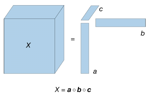
Rank-One Tensor
A Rank-One Tensor can be created by the outer product of multiple vectors, e.g., a 3-order rank-one tensor is obtained by
Candecomp/Parafac (CP) Decomposition
Candecomp/Parafac (CP)(Parallel Factor Analysis) decomposition is a tensor decomposition method used in multilinear algebra and multivariate data analysis. It is an extension of the matrix factorization technique, like Singular Value Decomposition (SVD), to higher-order tensors, often referred to as multi-way arrays.
The CP decomposition factorizes a tensor into a sum of component rank-one tensors, e.g. given a third-order tensor $X \in R^{I \times J\ times K}$, CP decomposition is given by,
$X \approx \sum_{r=1}^{R} a_r \cdot b_r \cdot c_r$
$R$ is a positive integer.
If R is the rank of higher-tensor then CP decomposition will be exact and unique.
Rank of Tensor
Rank of a tensor $X$, denoted by $rank(X)$ is the smallest number of rank-one tensors whose sum can generate $X$
Determining the rank of a tensor is an NP-hard problem. Some weaker upper bounds, however, exits that helps restrict the rank space. For example,
$X^{I \times J \times K}$,
$rank(X)$ $\le min(IJ,JK, IK)$
CP Decomposition in Python
import numpy as np
import tensorly as tl

# Define the dimensions of the tensor
I = 3
J = 4
K = 5

# Create a random tensor with the specified dimensions
X = np.random.rand(I, J, K)

# Set the desired rank for the decomposition
rank = 2

# Perform CP decomposition using TensorLy
factors = tl.decomposition.parafac(X, rank=rank)

# Reconstruct the original tensor
reconstructed_X = tl.kruskal_to_tensor(factors)

# Evaluate the reconstruction error
reconstruction_error = tl.norm(X - reconstructed_X, 2)
print(f'Reconstruction Error: {reconstruction_error}')
Tucker Decomposition
Tucker Decomposition is not a special case of CP Decomposition
Tucker decomposition, also known as Tucker factorization or Tucker model, is a tensor decomposition method used to represent a multi-dimensional tensor as a core tensor and a set of factor matrices that capture the relationships between the tensor’s modes or dimensions. Tucker decomposition is a higher-order extension of matrix factorization techniques like Singular Value Decomposition (SVD) to tensors.
In Tucker decomposition, a given tensor is approximated as the product of a core tensor and a set of factor matrices for each mode. The core tensor contains the most important information about the original tensor’s structure, while the factor matrices capture how each mode contributes to the overall tensor. Here’s an overview of the Tucker decomposition process:
import tensorly as tl
import numpy as np

# Define the dimensions of the tensor
shape = (3, 4, 5)  # Change these dimensions according to your data

# Create a random tensor with the specified dimensions
X = tl.tensor(np.random.rand(*shape))

# Specify the Tucker rank (adjust these values as needed)
rank = (2, 2, 2)

# Perform Tucker decomposition using TensorLy
core, factors = tl.decomposition.tucker(X, rank=rank)

# Reconstruct the original tensor
reconstructed_X = tl.tucker_to_tensor(core, factors)

# Evaluate the reconstruction error
reconstruction_error = tl.norm(X - reconstructed_X, 2)
print(f'Reconstruction Error: {reconstruction_error}')
Optimization and Application
In plain English, optimization is the action of making the best or most effective use of a situation or resource. Optimization problems are of great practical interest. For example, in manufacturing, how should one cut plates of a material so that the waste is minimized? In business, how should a company allocate the available resources that its profit is maximized? Some of the first optimization problems have been solved in ancient Greece and are regarded among the most significant discoveries of that time. In the first century A.D., the Alexandrian mathematician Heron solved the problem of finding the shortest path between two points by way of the mirror.
This result, also known as Heron’s theorem of the light ray, can be viewed as the origin of the theory of geometrical optics. The problem of finding extreme values gained special importance in the seventeenth century, when it served as one of the motivations in the invention of differential calculus, which is the foundation of the modern theory of mathematical optimization.
Generic form of optimization problem:
$min$ $f(x)$ $s.t.$ $x \in X $
- The vector $x = (x_1, . . . , x_n)$ is the optimization variable (or decision variable) of the problem
- The function $f$ is the objective function
- A vector $x$ is called optimal, or a solution (not optimal solution) of the problem, if it has the smallest objective value among all vectors that satisfy the constraints
- $X$ is the set of inequality constraints
Mathematical ingredients:
- Encode decisions/actions as decision variables whose values we are seeking
- Identify the relevant problem data
- Express constraints on the values of the decision variables as mathematical relationships (inequalities) between the variables and problem data
- Express the objective function as a function of the decision variables and the problem data.
Minimize or Maximize an objective function of decision variable subject to constraints on the values of the decision variables.
min or max f(x1, x2, .... , xn)
subject to gi(x1, x2, ...., ) <= bi     i = 1,....,m
        xj is continuous or discrete    j = 1,....,n
The problem setting
- Finite number of decision variables
- A single objective function of decision variables and problem data
- Multiple objective functions are handled by either taking a weighted combination of them or by optimizing one of the objectives while ensuring the other objectives meet target requirements.
- The constraints are defined by a finite number of inequalities or equalities involving functions of the decision variables and problem data
- There may be domain restrictions (continuous or discrete) on some of the variables
- The functions defining the objective and constraints are algebraic (typically with rational coefficients)
Minimization vs Maximization
- Without the loss of generality, it is sufficient to consider a minimization objective since maximization of objective function is minimization of the negation of the objective function
Program vs Optimization
- A program or mathematical program is an optimization problem with a finite number of variables and constraints written out using explicit mathematical (algebraic) expressions
- The word program means plan/planning
- Early application of optimization arose in planning resource allocations and gave rise to programming to mean optimization (predates computer programming)
Example: Designing a box:
Given a $1$ feet by $1$ feet piece of cardboard, cut out corners and fold to make a box of maximum volume:
Decision: $x$ = how much to cut from each of the corners?
Alternatives: $0<=x<=1/2$
Best: Maximize volume: $V(x) = x(1-2x)^2$ ($x$ is the height and $(1-2x)^2$ is the base, and their product is the volume)
Optimization formulation: $max$ $x(1-2x)^2$ subject to $0<=x<=1/2$ (which are the constraints in this case)
This is an unconstrained optimization problem since the constraint is a simple bound based.
Example: Data Fitting:
Given $N$ data points $(y_1, x_1)…(y_N, x_N)$ where $y_i$ belongs to $\mathbb{R}$ and $x_i$ belongs to $\mathbb{R}^n$, for all $i = 1..N$, find a line $y = a^Tx+b$ that best fits the data.
Decision: A vector $a$ that belongs to $\mathbb{R}^n$ and a scalar $b$ that belongs to $\mathbb{R}$
Alternatives: All $n$-dimensional vectors and scalars
Best: Minimize the sum of squared errors
Optimization formulation:
$\begin{array}{ll}\min & \sum_{i=1}^N\left(y_i-a^{\top} x_i-b\right)^2 \ \text { s.t. } & a \in \mathbb{R}^n, b \in \mathbb{R}\end{array}$
This is also an unconstrained optimization problem.
Example: Product Mix:
A firm make $n$ different products using $m$ types of resources. Each unit of product $i$ generates $p_i$ dollars of profit, and requires $r_{ij}$ units of resource $j$. The firm has $u_j$ units of resource $j$ available. How much of each product should the firm make to maximize profits?
Decision: how much of each product to make
Alternatives: defined by the resource limits
Best: Maximize profits
Optimization formulation:
Sum notation: $\begin{array}{lll}\max & \sum_{i=1}^n p_i x_i \ \text { s.t. } & \sum_{i=1}^n r_{i j} x_i \leq u_j & \forall j=1, \ldots, m \ & x_i \geq 0 & \forall i=1, \ldots, n\end{array}$
Matrix notation: $\begin{array}{cl}\max & p^{\top} x \ \text { s.t. } & R x \leq u \ & x \geq 0\end{array}$
Example: Project investment
A firm is considering investing in $n$ different R&D projects. Project $j$ requires an investment of $c_j$ dollars and promises a return of $r_j$ dollars. The firm has a budget of $B$ dollars. Which projects should the firm invest in?
Decision: Whether or not to invest in project
Alternatives: Defined by budget
Best: Maximize return on investment
Sum notation: $\begin{aligned} \max & \sum_{j=1}^n r_j x_j \ \text { s.t. } & \sum_{j=1}^n c_j x_j \leq B \ & x_j \in{0,1} \forall j=1, \ldots, n\end{aligned}$
Matrix notation: $\begin{aligned} \max & r^{\top} x \ \text { s.t. } & c^{\top} x \leq B \ & x \in{0,1}^n\end{aligned}$
This is not an unconstrained problem.
- Identify basic portfolio optimization and associated issues
- Examine the Markowitz Portfolio Optimization approach
- Markowitz Principle: Select a portfolio that attempts to maximize the expected return and minimize the variance of returns (risk)
- For multi objective problem (like defined by the Markowitz Principle), two objectives can be combined:
- Maximize Expected Return - $\lambda$*risk
- Maximize Expected Return subject to risk <= s_max (constraint on risk)
- Minimize Risk subject to return >= r_min (threshold on expected returns)
- Optimization Problem Statement
Given $1000, how much should we invest in each of the three stocks MSFT, V and WMT so as to :
- have a one month expected return of at least a given threshold
- minimize the risk(variance) of the portfolio return
- Decision: investment in each stock
- alternatives: any investment that meets the budget and the minimum expected return requirement
- best: minimize variance
- Key trade-off: How much of the detail of the actual problem to consider while maintaining computational tractability of the mathematical model?
- Requires making simplifying assumptions, either because some of the problem characteristics are not well-defined mathematically, or because we wish to develop a model that can actually be solved
- Need to exercise great caution in these assumptions and not loose sight of the true underlying problem
- Assumptions:
- No transaction cost
- Stocks does not need to be bought in blocks (any amount >=0 is fine)
- Optimization Process: Decision Problem -> Model -> Data Collection -> Model Solution -> Analysis -> Problem solution
- No clear cut recipe
- Lots of feedbacks and iterations
- Approximations and assumptions involved in each stage
- Success requires good understanding of the actual problem (domain knowledge is important)
Classification of optimization problems
- The tractability of a large scale optimization problem depends on the structure of the functions that make up the objective and constraints, and the domain restrictions on the variables.
| Functions | Variable domains | Problem Type | Difficulty |
|---|---|---|---|
| All linear | Continuous variables | Linear Program | Easy |
| Some nonlinear | Continuous variables | Nonlinear Program or Nonlinear Optimization Problem | Easy/Difficult |
| Linear/nonlinear | Some discrete | Integer Problem or Discrete Optimization Problem | Difficult |
| Optimization Problem | Description | Difficulty |
|---|---|---|
| Linear Programming | A linear programming problem involves maximizing or minimizing a linear objective function subject to a set of linear constraints | Easy to moderate |
| Nonlinear Programming | A nonlinear programming problem involves optimizing a function that is not linear, subject to a set of nonlinear constraints | Moderate to hard |
| Quadratic Programming | A quadratic programming problem involves optimizing a quadratic objective function subject to a set of linear constraints | Moderate |
| Convex Optimization | A convex optimization problem involves optimizing a convex function subject to a set of linear or convex constraints | Easy to moderate |
| Integer Programming | An integer programming problem involves optimizing a linear or nonlinear objective function subject to a set of linear or nonlinear constraints, where some or all of the variables are restricted to integer values | Hard |
| Mixed-integer Programming | A mixed-integer programming problem is a generalization of integer programming where some or all of the variables can be restricted to integer values or continuous values | Hard |
| Global Optimization | A global optimization problem involves finding the global optimum of a function subject to a set of constraints, which may be nonlinear or non-convex | Hard |
| Stochastic Optimization | A stochastic optimization problem involves optimizing an objective function that depends on random variables, subject to a set of constraints | Hard |
Subclasses of NLP (Non Linear Problem)
- Unconstrained optimization: No constraints or simple bound constraints on the variables (Box design example above)
- Quadratic programming: Objectives and constraints involve quadratic functions (Data fitting example above), subset of NLP
Subclasses of IP (Integer Programming)
- Mixed Integer Linear Program
- All linear functions
- Some variables are continuous and some are discrete
- Mixed Integer Nonlinear Program (MINLP)
- Some nonlinear functions
- Some variables are continuous and some are discrete
- Mixed Integer Quadratic Program (MIQLP)
- Nonlinear functions are quadratic
- Some variables are continuous and some are discrete
- subset of MINLP
Why and how to classify?
- Important to recognize the type of an optimization problem:
- to formulate problems to be amenable to certain solution methods
- to anticipate the difficulty of solving the problem
- to know which solution methods to use
- to design customized solution methods
- how to classify:
- check domain restriction on variables
- check the structure of the functions involved
Taylor Approximation
The Taylor series of a real or complex-valued function f (x) that is infinitely differentiable at a real or complex number a is the power series.
Let $f: \mathbb{R}^n \rightarrow \mathbb{R}$ be a differentiable function and $\mathbf{x}^0 \in \mathbb{R}^n$.
- First order Taylor’s approximation of $f$ at $\mathbf{x}^0$ : $$ f(\mathbf{x}) \approx f\left(\mathbf{x}^0\right)+\nabla f\left(\mathbf{x}^0\right)^{\top}\left(\mathbf{x}-\mathbf{x}^0\right) $$
- Second order Taylor’s approximation of $f$ at $\mathbf{x}^0$ : $$ f(\mathbf{x}) \approx f\left(\mathbf{x}^0\right)+\nabla f\left(\mathbf{x}^0\right)^{\top}\left(\mathbf{x}-\mathbf{x}^0\right)+\frac{1}{2}\left(\mathbf{x}-\mathbf{x}^0\right)^{\top} \nabla^2 f\left(\mathbf{x}^0\right)\left(\mathbf{x}-\mathbf{x}^0\right) $$ `
Sets in Optimization Problems
- A set is closed if it includes its boundary points.
- Intersection of closed sets is closed.
- Typically, if none of inequalities are strict, then the set is closed.
- A set is convex if a line segment connecting two points in the set lies entirely in the set.
- A set is bounded if it can be enclosed in a large enough (hyper)-sphere or a box.
- A set that is both bounded and closed is called compact.
- $R^2$ is closed but not bounded
- $x^2+y^2<1$ is bounded but not closed
- $x+y>=1$ is closed but not bounded
- $x^2+y^2<=1$ is closed and bounded (compact)
- An optimal solution of maximizing a convex function over a compact set lies on the boundary of the set.
Convex Function

- A function $f: \mathbb{R}^n \rightarrow \mathbb{R}$ is convex if $$ f(\lambda \mathbf{x}+(1-\lambda) \mathbf{y}) \leq \lambda f(\mathbf{x})+(1-\lambda) f(\mathbf{y}) \quad \forall \mathbf{x}, \mathbf{y} \in \mathbb{R}^n \text { and } \lambda \in[0,1] $$
- “Function value at the average is less than the average of the function values”
- This also implies that $a^Tx+b$ is convex (and concave)
- For a convex function the first order Taylor’s approximation is a global under estimator
- A convex optimization problem has a convex objective and convex set of solutions.
- Linear programs (LPs) can be seen as a special case of convex optimization problems. In an LP, the objective function and constraints are linear, which means that the feasible region defined by the constraints is a convex set. As a result, the optimal solution to an LP is guaranteed to be at a vertex (corner) of the feasible region, which makes it a convex optimization problem.
- A twice differentiable univariate function is convex if $f^{’’}(x)>=0$ for all $x \in R$
- To generalize, a twice differentiable function is convex if and only if the Hessian matrix is positive semi definite.
- A positive semi-definite (PSD) matrix is a matrix that is symmetric and has non-negative eigenvalues. In the context of a Hessian matrix, it represents the second-order partial derivatives of a multivariate function and reflects the curvature of the function. If the Hessian is PSD, it indicates that the function is locally convex, meaning that it has a minimum value in the vicinity of that point. On the other hand, if the Hessian is not PSD, the function may have a saddle point or be locally non-convex. The PSD property of a Hessian matrix is important in optimization, as it guarantees the existence of a minimum value for the function.
- Sylvester’s criterion is a method for determining if a matrix is positive definite or positive semi-definite. The criterion states that a real symmetric matrix is positive definite if and only if all of its leading principal minors (i.e. determinants of the submatrices formed by taking the first few rows and columns of the matrix) are positive. If all the leading principal minors are non-negative, then the matrix is positive semi-definite.
First Order Methods
Gradient descent
Gradient descent is an iterative optimization algorithm used to find the minimum of a function, typically used in machine learning and deep learning to update the parameters of a model during training. The basic idea behind gradient descent is to adjust the parameters in the direction of steepest descent (negative gradient) to minimize a cost or loss function. Here’s a detailed explanation of gradient descent:
- Objective Function : Gradient descent begins with an objective function (also called a cost or loss function) that you want to minimize. In machine learning, this function typically represents the error between the model’s predictions and the actual data.
Let’s denote the objective function as $J(θ)$, where $θ$ represents a vector of parameters that we want to optimize.
-
Initialization : You start by initializing the parameter vector θ with some arbitrary values or often with random values. This is the starting point of the optimization process.
-
Gradient Calculation : Calculate the gradient of the objective function with respect to the parameters. The gradient is a vector that points in the direction of the steepest increase in the function. Mathematically, the gradient is represented as:
$(\nabla J(\theta) = \left[\frac{\partial J(\theta)}{\partial \theta_1}, \frac{\partial J(\theta)}{\partial \theta_2}, \ldots, \frac{\partial J(\theta)}{\partial \theta_n}\right]) $
Here, $∂J(θ)/∂θ_i$ represents the partial derivative of $J(θ)$ with respect to the i-th parameter $θ_i$.
- Update Parameters : Update the parameters θ using the gradient. The update rule is as follows:
$θ_{new} = θ_{old} - α * ∇J(θ_{old})$
Where:
- $θ_{new}$ is the updated parameter vector.
- $θ_{old}$ is the current parameter vector.
- $α$ (alpha) is the learning rate, a hyperparameter that controls the step size or how much to move in the direction of the gradient. It’s a small positive value typically chosen in advance.
This step is performed iteratively until a stopping criterion is met.
-
Stopping Criterion : The algorithm continues to update the parameters and compute the gradient until a stopping criterion is satisfied. Common stopping criteria include a maximum number of iterations, a minimum change in the objective function, or when the gradient becomes close to zero.
-
Convergence : Gradient descent converges when it reaches a local or global minimum of the objective function, or when it satisfies the stopping criterion. The choice of learning rate (α) and the convergence behavior are important aspects to consider when using gradient descent.
There are variations of gradient descent, including:
- Batch Gradient Descent : In each iteration, it computes the gradient using the entire dataset. This can be computationally expensive for large datasets.
- Stochastic Gradient Descent (SGD) : In each iteration, it computes the gradient using only one random data point from the dataset. It’s faster but has more noise in its updates.
- Mini-batch Gradient Descent : It uses a small random subset (mini-batch) of the dataset in each iteration, striking a balance between the computational efficiency of SGD and the stability of batch gradient descent.
- Momentum, Adagrad, RMSprop, and Adam : These are advanced optimization techniques that incorporate additional mechanisms to improve convergence speed and stability.
The choice of the specific gradient descent variant and its hyperparameters depends on the problem at hand, the dataset, and computational resources. Proper tuning of the learning rate and monitoring convergence is crucial for successful optimization.
import numpy as np

def gradient_descent(obj_func, gradient_func, initial_theta, learning_rate=0.01, max_iterations=1000, tolerance=1e-5):
    theta = initial_theta
    for iteration in range(max_iterations):
        gradient = gradient_func(theta)
        theta = theta - learning_rate * gradient

        # Calculate the magnitude of the gradient for convergence check
        gradient_magnitude = np.linalg.norm(gradient)

        if gradient_magnitude < tolerance:
            print(f"Converged after {iteration} iterations.")
            break

    return theta

def objective_function(theta):
    return theta[0]**2 + theta[1]**2

def gradient_function(theta):
    return np.array([2 * theta[0], 2 * theta[1]])

# Initial parameters
initial_theta = np.array([3.0, 4.0])

# Call gradient descent
final_theta = gradient_descent(objective_function, gradient_function, initial_theta)

print("Optimal parameters:", final_theta)
print("Minimum value of the objective function:", objective_function(final_theta))
Accelerated Gradient Descent
Accelerated Gradient Descent, also known as Nesterov Accelerated Gradient (NAG) or simply Nesterov momentum, is an optimization algorithm that improves upon the standard gradient descent by adding momentum to the updates. This momentum helps the algorithm converge faster and provides better stability, especially in the presence of noisy gradients. Here’s how it works:
- Initialization : Initialize the parameter vector θ with some arbitrary values, and initialize the momentum vector
vto zero. - Update Momentum (v) : In each iteration, before computing the gradient, update the momentum vector
vusing the previous momentum and the gradient from the previous iteration. This is the key difference between NAG and traditional momentum.
$v_t = γ * v_{t-1} + α * ∇J(θ_{t-1} - γ * v_{t-1})$
- $γ$ is the momentum coefficient (typically a value close to 0.9).
- $α$ is the learning rate.
- $∇J(θ_{t-1} - γ * v_{t-1})$ is the gradient of the loss function evaluated at the updated position using the momentum.
- Update Parameters (θ) : Update the parameters θ using the momentum
vcomputed in the previous step.
$θ_t = θ_{t-1} - v_t$
- Repeat : Repeat steps 2 and 3 until a stopping criterion is met, such as a maximum number of iterations or a small gradient magnitude.
The key insight in Nesterov Accelerated Gradient Descent is that it calculates the gradient at a “lookahead” position by subtracting the previous momentum-scaled update from the current parameters before computing the gradient. This lookahead helps in achieving smoother convergence by reducing oscillations.
Here’s a Python implementation of Nesterov Accelerated Gradient Descent:
import numpy as np

def nesterov_accelerated_gradient_descent(obj_func, gradient_func, initial_theta, learning_rate=0.01, momentum=0.9, max_iterations=1000, tolerance=1e-5):
    theta = initial_theta
    v = np.zeros_like(initial_theta)

    for iteration in range(max_iterations):
        gradient = gradient_func(theta - momentum * v)
        v = momentum * v + learning_rate * gradient
        theta = theta - v

        # Calculate the magnitude of the gradient for convergence check
        gradient_magnitude = np.linalg.norm(gradient)

        if gradient_magnitude < tolerance:
            print(f"Converged after {iteration} iterations.")
            break

    return theta

# Example usage:
# Define your objective function and gradient function
def objective_function(theta):
    return theta[0]**2 + theta[1]**2

def gradient_function(theta):
    return np.array([2 * theta[0], 2 * theta[1]])

# Initial parameters
initial_theta = np.array([3.0, 4.0])

# Call Nesterov Accelerated Gradient Descent
final_theta = nesterov_accelerated_gradient_descent(objective_function, gradient_function, initial_theta)

print("Optimal parameters:", final_theta)
print("Minimum value of the objective function:", objective_function(final_theta))
In this implementation, momentum is the momentum coefficient (typically close to 0.9), and learning_rate is the step size. The rest of the algorithm follows the Nesterov Accelerated Gradient Descent procedure described earlier.
Stochastic Gradient Descent (SGD)
Stochastic Gradient Descent (SGD) is an optimization algorithm used for training machine learning models, particularly in cases where you have a large dataset. Unlike traditional gradient descent, which computes the gradient of the cost function using the entire dataset in each iteration, SGD updates the model’s parameters by considering only a single randomly chosen data point (or a small batch of data points) in each iteration. This makes it much faster and enables it to handle large datasets.
Here’s how Stochastic Gradient Descent works:
- Initialization : Start with an initial guess for the model’s parameters, often set to small random values.
- Shuffling : Shuffle the training dataset randomly. This step ensures that the data points are processed in a random order in each epoch (a complete pass through the dataset).
- Iterative Update : For each iteration:
- Select a random data point (or a small mini-batch) from the shuffled dataset.
- Compute the gradient of the loss function with respect to the model’s parameters using only the selected data point (or mini-batch).
- Update the model’s parameters in the opposite direction of the gradient:
$θ = θ - learningrate * gradient$
Where:
θrepresents the model’s parameters.learningrateis a positive scalar called the learning rate, which controls the step size in the parameter update.gradientis the gradient of the loss function with respect to the parameters computed using the selected data point (or mini-batch).
- Repeat : Continue this process for a fixed number of iterations (epochs) or until a stopping criterion is met.
SGD has several advantages, including:
- Efficiency: It’s computationally efficient because it uses only one or a few data points at a time, making it suitable for large datasets.
- Regularization: The inherent randomness in SGD acts as a form of regularization, which can help prevent overfitting.
- Escape Local Minima: The noise introduced by using individual data points can help the algorithm escape local minima in the loss landscape.
However, SGD can have high variance in its parameter updates because of the noisy gradient estimates, which can lead to oscillations and slow convergence. To address this, variations of SGD have been developed, including Mini-batch Gradient Descent, which uses small random mini-batches of data, and techniques like learning rate schedules and momentum to stabilize and accelerate convergence.
Here’s a simple Python implementation of Stochastic Gradient Descent:
import numpy as np

def stochastic_gradient_descent(obj_func, gradient_func, initial_theta, learning_rate=0.01, max_epochs=1000, tolerance=1e-5):
    theta = initial_theta
    num_examples = len(obj_func)  # Number of data points

    for epoch in range(max_epochs):
        # Shuffle the data for each epoch
        shuffled_indices = np.random.permutation(num_examples)
        for i in shuffled_indices:
            gradient = gradient_func(theta, i)
            theta = theta - learning_rate * gradient

            # Calculate the magnitude of the gradient for convergence check
            gradient_magnitude = np.linalg.norm(gradient)

            if gradient_magnitude < tolerance:
                print(f"Converged after {epoch} epochs.")
                return theta

    print("Did not converge.")
    return theta

# Initial parameters
initial_theta = np.array([3.0, 4.0])

# Call Stochastic Gradient Descent
final_theta = stochastic_gradient_descent(obj_func, gradient_func, initial_theta)

print("Optimal parameters:", final_theta)
print("Minimum value of the objective function:", obj_func(final_theta))
In this implementation, obj_func represents the objective function you want to minimize, and gradient_func computes the gradient of the loss function with respect to the model’s parameters for a specific data point i. The rest of the algorithm follows the SGD procedure described earlier.
Second order Methods
Newton method
Newton-Raphson method, often referred to as the Newton method, is an iterative numerical technique used to find the approximate roots (or solutions) of real-valued functions. It is particularly effective for finding the roots of nonlinear equations, optimizing functions, and solving systems of nonlinear equations. The method is named after Sir Isaac Newton and Joseph Raphson, who contributed to its development.
The basic idea behind the Newton method is to iteratively refine an initial guess for the root by approximating the function with a linear equation (a tangent line) near the current guess. Mathematically, the algorithm can be summarized as follows:
Given a function $f(x)$ and an initial guess $x_0$, repeat the following steps until a convergence criterion is met:
- Compute the value of the function $f(x_n)$ and its derivative $f′(x_n)$ at the current guess $x_n$.
- Update the guess for the root using the formula: $(x_{n+1} = x_{n} - \frac{f’(x_{n})}{f(x_{n})})$
- Repeat steps 1 and 2 until $∣f(xn+1)∣$ is sufficiently close to zero or until a maximum number of iterations is reached.
The method converges rapidly if the initial guess is reasonably close to the actual root and if the function is well-behaved (continuous and with a well-defined derivative).
Here’s a Python implementation of the Newton method to find the root of a single-variable function:
def newton_method(f, df, x0, tol=1e-6, max_iter=100):
    x = x0
    for iteration in range(max_iter):
        fx = f(x)
        dfx = df(x)

        # Check for small derivatives to avoid division by zero
        if abs(dfx) < 1e-6:
            raise ValueError("Derivative is too small.")

        x_new = x - fx / dfx

        if abs(x_new - x) < tol:
            print(f"Converged after {iteration} iterations.")
            return x_new

        x = x_new

    print("Did not converge.")
    return None

# Example usage:
# Define your function f(x) and its derivative df(x)
def f(x):
    return x**2 - 4

def df(x):
    return 2 * x

# Initial guess
x0 = 3.0

# Call Newton's method
root = newton_method(f, df, x0)

print("Approximate root:", root)
In this example, f(x) represents the function you want to find the root of, and df(x) is its derivative. The algorithm iteratively refines the estimate of the root (x) until it converges within a specified tolerance (tol) or until a maximum number of iterations (max_iter) is reached.
Gauss-Newton method
Gauss-Newton method iteratively updates the parameter vector ppp to minimize the objective function. In each iteration, it approximates the objective function using a linearization around the current estimate of ppp, which is why it’s often considered an extension of the Newton-Raphson method for nonlinear optimization.
Here are the main steps of the Gauss-Newton method:
- Initialization : Start with an initial guess for the parameter vector ppp.
- Iterative Update:
- For each iteration:
- Calculate the Jacobian matrix $J(p)$, which contains the partial derivatives of the model predictions $f_i(p)$ with respect to each parameter.
- Calculate the residual vector $r(p)$, which is the difference between the observed data $y_i$ and the model predictions $f_i(p)$ for all data points.
- Update the parameter vector $p$ using the following formula: $p_{\text{new}} = p_{\text{old}} + \Delta p$ where $\Delta p = (J^T J)^{-1} J^T r$ $J^T$ is the transpose of the Jacobian matrix, and $(J^T J)^{-1}$ is the pseudoinverse of the Jacobian matrix.
- Repeat the iterative update until a convergence criterion is met, such as small changes in the parameter estimates or a maximum number of iterations.
- For each iteration:
- Convergence: The algorithm converges when the parameter estimates $p$ stabilize or when a predefined stopping criterion is satisfied.
Here’s a Python example demonstrating the Gauss-Newton method for nonlinear regression:
import numpy as np
from scipy.optimize import least_squares

# Define the model function and its Jacobian
def model(p, x):
    return p[0] * np.exp(-p[1] * x)

def jacobian(p, x):
    return np.vstack((-np.exp(-p[1] * x), x * p[0] * np.exp(-p[1] * x))).T

# Generate synthetic data
np.random.seed(0)
x_data = np.linspace(0, 2, 100)
true_params = [2.0, 1.0]
y_data = model(true_params, x_data) + 0.1 * np.random.randn(len(x_data))

# Define the objective function (residuals)
def objective(p):
    return y_data - model(p, x_data)

# Initial guess for parameters
initial_guess = [1.0, 2.0]

# Use SciPy's least_squares function to perform Gauss-Newton optimization
result = least_squares(objective, initial_guess, jac=jacobian, method='lm')

# Extract the estimated parameters
estimated_params = result.x

print("True parameters:", true_params)
print("Estimated parameters:", estimated_params)
In this example, we define a simple exponential model and generate synthetic data with added noise. Then, we use SciPy’s least_squares function to perform the Gauss-Newton optimization to estimate the parameters of the model. The estimated parameters are compared to the true parameters to assess the quality of the fit.
Quasi-Newton methods
Quasi-Newton methods are a class of optimization algorithms used for finding the minimum of a scalar function of several variables. These methods belong to the broader category of gradient-based optimization techniques and are particularly useful when it’s computationally expensive to compute the exact Hessian matrix (the matrix of second derivatives) of the objective function. Instead of calculating the Hessian directly, quasi-Newton methods approximate it using updates based on gradient information, making them more efficient for many practical optimization problems.
The most well-known quasi-Newton method is the Broyden–Fletcher–Goldfarb–Shanno (BFGS) algorithm, but there are other variants like the Limited-memory BFGS (L-BFGS) that are suitable for large-scale problems. Here’s an overview of how quasi-Newton methods work:
- Initialization : Start with an initial guess for the parameters (variables) you want to optimize.
- Initialization of the Approximate Hessian : Initialize an approximation of the Hessian matrix. In BFGS, for example, this is usually done with the identity matrix or a scaled version of it.
- Iterative Update : Quasi-Newton methods iteratively update the parameter vector and the approximation of the Hessian matrix until convergence is achieved. The main steps in each iteration are as follows:
- Calculate the Gradient : Compute the gradient of the objective function with respect to the parameters at the current parameter values.
- Solve the Quasi-Newton Equation : Quasi-Newton methods update the approximation of the Hessian matrix using information from the gradient and parameter changes. The update formula depends on the specific quasi-Newton method (e.g., BFGS or L-BFGS). The objective is to construct an approximation of the Hessian that preserves important curvature information of the objective function.
- Update Parameters : Update the parameter vector using the approximate Hessian matrix. This update step usually involves solving a linear system of equations that is determined by the approximation of the Hessian.
- Convergence Check : Check for convergence criteria, such as the magnitude of the gradient, small changes in the parameters, or a predefined number of iterations.
- Convergence : The optimization process terminates when one or more convergence criteria are met.
Quasi-Newton methods are efficient and widely used because they can handle large-scale optimization problems without explicitly computing and storing the full Hessian matrix, which can be computationally expensive and memory-intensive. Instead, they maintain an approximation of the Hessian using a limited amount of memory.
Here’s an example of how to use the L-BFGS-B variant of the L-BFGS quasi-Newton method in Python using SciPy’s optimization module:
import numpy as np
from scipy.optimize import minimize

# Define the objective function to minimize
def objective_function(x):
    return (x[0] - 2) ** 2 + (x[1] - 3) ** 2

# Initial guess for the parameters
initial_guess = [0.0, 0.0]

# Use L-BFGS-B for optimization
result = minimize(objective_function, initial_guess, method='L-BFGS-B')

# Extract the optimized parameters
optimized_parameters = result.x

print("Optimized parameters:", optimized_parameters)
print("Minimum value of the objective function:", result.fun)
In this example, we define a simple quadratic objective function to minimize, and we use the minimize function from SciPy’s optimization module with the L-BFGS-B method to find the minimum. The result object contains the optimized parameters and the minimum value of the objective function.
Proximal Gradient Descent
Proximal Gradient Descent is a method used in optimization, particularly for handling problems where the objective function is composed of two parts. The first part is convex and continious, whereas the second part is convex but not continious.
Implementation of Proximal Gradient Descent in Python for LASSO:
import numpy as np

def soft_thresholding(v, lambda_alpha):
    return np.sign(v) * np.maximum(np.abs(v) - lambda_alpha, 0)

def proximal_gradient_descent(X, y, alpha, lambda_=1e-3, n_iter=100):
    m, n = X.shape
    beta = np.zeros(n)

    for _ in range(n_iter):
        # Gradient step
        gradient = -np.dot(X.T, y - np.dot(X, beta)) / m
        beta = beta - lambda_ * gradient

        # Proximal step (for L1 norm)
        beta = soft_thresholding(beta, lambda_ * alpha)

    return beta


X = np.random.rand(100, 10)
y = np.random.rand(100)
alpha = 0.1

beta = proximal_gradient_descent(X, y, alpha)
print(beta)
Accelerated Proximal Gradient Descent
import numpy as np

def soft_thresholding(v, lambda_alpha):
    return np.sign(v) * np.maximum(np.abs(v) - lambda_alpha, 0)

def accelerated_proximal_gradient_descent(X, y, alpha, lambda_=1e-3, n_iter=100):
    m, n = X.shape
    x = np.zeros(n)
    y = x.copy()
    t = 1

    for _ in range(n_iter):
        old_x = x.copy()
        gradient = -np.dot(X.T, y - np.dot(X, y)) / m
        x = y - lambda_ * gradient
        x = soft_thresholding(x, lambda_ * alpha)
        t_old = t
        t = (1 + np.sqrt(1 + 4 * t ** 2)) / 2
        y = x + ((t_old - 1) / t) * (x - old_x)

    return x


X = np.random.rand(100, 10)
y = np.random.rand(100)
alpha = 0.1

beta = accelerated_proximal_gradient_descent(X, y, alpha)
print(beta)
Augmented Lagrangian Method and Alternating Direction Methods for Multipliers
- Proximal gradient descent is useful for minimizing decomposable convex functions with a differentiable and a non-differentiable part
- However if prox is not easy to obtain, proximal gradient methods may not be useful.
- Augmented Lagrangian Method and Alternating Direction Methods for Multipliers can be useful here
import numpy as np

# Objective function
def f(x):
    return x[0]**2 + x[1]**2

# Constraint (should return zero when constraint is satisfied)
def h(x):
    return x[0] + x[1] - 1

# Gradient of the objective function
def grad_f(x):
    return 2 * x

# Gradient of the constraint function
def grad_h(x):
    return np.array([1, 1])

# Augmented Lagrangian function
def L_A(x, lambda_, rho):
    return f(x) + lambda_ * h(x) + (rho / 2) * h(x)**2

# Gradient of the Augmented Lagrangian
def grad_L_A(x, lambda_, rho):
    return grad_f(x) + lambda_ * grad_h(x) + rho * h(x) * grad_h(x)

# Simple Gradient Descent for the x-update step
def gradient_descent_update(x, lambda_, rho, learning_rate=0.01):
    return x - learning_rate * grad_L_A(x, lambda_, rho)

# Augmented Lagrangian Method
def augmented_lagrangian_method(initial_x, initial_lambda, rho, max_iter=100):
    x = initial_x
    lambda_ = initial_lambda

    for i in range(max_iter):
        x = gradient_descent_update(x, lambda_, rho)
        lambda_ = lambda_ + rho * h(x)  # λ-update

    return x

# Example usage
x_opt = augmented_lagrangian_method(np.array([0, 0]), 0, 10)
print("Optimized x:", x_opt)
ADMM
- Similar to Augmented Lagrangian method, we augment the objective function.
- The augmented term does not change the objective, as its value is always zero due to the constraints.
import numpy as np

def admm(f, g, A, B, c, rho, max_iter=100):
    x = np.zeros(A.shape[1])
    z = np.zeros(B.shape[1])
    lambda_ = np.zeros(c.shape)

    for _ in range(max_iter):
        # x-update (modify according to your f)
        x = np.linalg.inv(A.T @ A + rho * np.eye(A.shape[1])) @ (A.T @ (c - B @ z + lambda_/rho))

        # z-update (modify according to your g)
        z = np.linalg.inv(B.T @ B + rho * np.eye(B.shape[1])) @ (B.T @ (c - A @ x - lambda_/rho))

        # λ-update
        lambda_ = lambda_ + rho * (A @ x + B @ z - c)

    return x, z

# Example usage
A = np.array([[1, 2], [3, 4]])
B = np.array([[-1, 1], [2, -2]])
c = np.array([1, 0])

# Define f and g (here they are simple placeholders)
f = lambda x: np.linalg.norm(x, 2)
g = lambda z: np.linalg.norm(z, 2)

rho = 1.0
x, z = admm(f, g, A, B, c, rho)
print("x:", x)
print("z:", z)
Coordinate Descent Algorithm
Coordinate Descent is an optimization algorithm where the solution is obtained by successively optimizing the objective function along one direction or coordinate at a time. This approach is particularly effective for problems where each step of optimizing along a single coordinate (or a small block of coordinates) can be performed efficiently. Coordinate Descent is widely used in scenarios such as large-scale linear regression, LASSO regression, and machine learning algorithms where the dimensionality of the data is high.
import numpy as np

def coordinate_descent(A, b, lam, num_iters=1000, tol=1e-5):
    m, n = A.shape
    x = np.zeros(n)
    r = b - A.dot(x)

    for _ in range(num_iters):
        x_old = x.copy()

        for i in range(n):
            # Compute the update for coordinate i (assuming a quadratic objective)
            A_i = A[:, i]
            r += A_i * x[i]
            x[i] = np.dot(A_i, r) / (np.dot(A_i, A_i) + lam)
            r -= A_i * x[i]

        # Check for convergence
        if np.linalg.norm(x - x_old, ord=2) < tol:
            break

    return x

# Example usage
A = np.random.rand(100, 10)
b = np.random.rand(100)
lam = 1.0  # Regularization parameter

x = coordinate_descent(A, b, lam)
print(x)
Regularization
Regularization is a crucial technique in machine learning used to prevent overfitting and improve the generalization ability of a model. Overfitting occurs when a model learns the training data too well, including its noise and outliers, leading to poor performance on new, unseen data. Regularization helps to keep the model simple and more generalized by adding a penalty on the complexity of the model. The most common regularization techniques are:
- L1 Regularization (Lasso Regression): Adds a penalty equal to the absolute value of the magnitude of coefficients. This can lead to coefficients being zero, which is useful for feature selection in models where some features are irrelevant or redundant. L1 regularization tends to produce sparse solutions and is defined as:
Cost function+λ∑∣wi∣\text{Cost function} + \lambda \sum |w_i|Cost function+λ∑∣wi∣
Where λ\lambdaλ is a regularization parameter and wiw_iwi are the model weights. 2. L2 Regularization (Ridge Regression): Adds a penalty equal to the square of the magnitude of coefficients. This discourages large weights but does not force them to be zero, leading to a model where all features are considered but their impact is moderated. L2 regularization is defined as:
Cost function+λ∑wi2\text{Cost function} + \lambda \sum w_i^2Cost function+λ∑wi2
This method tends to distribute error among all the terms, but it doesn’t necessarily eliminate any weights completely, as L1 can. 3. Elastic Net: A combination of L1 and L2 regularization. It adds both penalties to the model and is useful when there are multiple features that are correlated with one another. Elastic Net aims to enjoy the benefits of both Ridge and Lasso regularization, allowing it to handle situations when there are numerous correlated features. 4. Early Stopping: A form of regularization used especially in neural networks where training is stopped as soon as the performance on a validation set starts to degrade. This prevents the model from learning the training data too well. 5. Dropout: Specifically used in neural networks, it involves randomly setting a fraction of input units to 0 at each update during training time, which helps prevent overfitting. This forces the network to not rely too much on any one node, hence aiding in generalization. 6. Max-Norm Regularization: In neural networks, this involves limiting the size of the weight vector for every neuron to a maximum value. This can be effective at preventing overfitting and is often used alongside dropout.
Ridge Regression ($L_2$)
Ridge regression is a technique used primarily to analyze multiple regression data that suffer from multicollinearity. When multicollinearity occurs, least squares estimates are unbiased, but their variances are large so they may be far from the true value. This can result in overfitting in the model, where the model performs well on the training data but poorly on unseen data.
Key Concepts in Ridge Regression:
- Shrinkage Penalty: The core idea of ridge regression is to introduce a regularization (shrinkage penalty) to the regression estimates. This method is also known as Tikhonov regularization. It works by penalizing the size of the regression coefficients.
- Cost Function: In ridge regression, the cost function is altered by adding a penalty equivalent to square of the magnitude of the coefficients. The regularization term is given by $λ$ (lambda), a tuning parameter multiplied by the sum of the squares of the coefficients:
$J(\theta) = \text{RSS} + \lambda \sum_{j=1}^{p} \theta_j^2$
Here, RSS is the residual sum of squares and $\theta$ represents the coefficient vector. The λ controls the amount of shrinkage: the larger the value of λ, the greater the amount of shrinkage.
- Bias-Variance Trade-off: By introducing $λ$, ridge regression trades off the unbiasedness of the OLS estimator for a reduction in variance, potentially leading to better mean squared error (MSE) on new observations. The coefficients are shrunk towards zero and towards each other, leading to a more stable and interpretable model.
- Solving Ridge Regression: The solution for the ridge estimate is:
$\hat{\beta}^{ridge} = (X^TX + \lambda I)^{-1}X^Ty$
where XXX is the matrix of input features, and III is the identity matrix. This formula shows how ridge regression penalizes the scale of the coefficients based on the value of λ.
-
Choice of λ: The value of λ is crucial in ridge regression. If λ = 0, the solution is just the ordinary least squares estimates. As λ → ∞, all coefficients are shrunk towards zero. The choice of λ is typically done via cross-validation, often seeking to minimize prediction error.
-
Geometric Interpretation: Geometrically, ridge regression constrains the coefficients to lie within a sphere centered at zero with radius proportional to 1/λ1/\sqrt{\lambda}1/λ. This constraint can lead to better prediction accuracy when the true relationship between the target and the predictors is approximately linear but complex, with predictors exhibiting collinearity.
-
Multicollinearity: Ridge regression doesn’t eliminate multicollinearity but mitigates its problematic aspects by controlling the coefficient magnitude and introducing bias into the estimates, which may improve prediction accuracy.
-
Applications: Ridge regression is widely used when the data has many multicollinear predictors and when prediction accuracy is a priority over interpretability. It’s also used in scenarios where the number of predictors exceeds the number of observations.
Statistics Form
$\min_{\beta} \sum_{i=1}^{n} (y_i - \beta_0 - \sum_{j=1}^{p} \beta_j x_{ij})^2 + \lambda \sum_{j=1}^{p} \beta_j^2$
Optimization Form
$\min_{\beta} { | \mathbf{y} - \mathbf{X}\beta |^2 + \lambda | \beta |^2 }$
Matrix Form
$| \mathbf{y} - \mathbf{X}\beta |^2 + \lambda | \beta |^2$ $\mathbf{X}^\top \mathbf{X}\beta + \lambda \mathbf{I}\beta = \mathbf{X}^\top \mathbf{y}$ $\beta = (\mathbf{X}^\top \mathbf{X} + \lambda \mathbf{I})^{-1} \mathbf{X}^\top \mathbf{y}$
Lasso Regression
The key aspects of Lasso regression include:
- Regularization Term: Lasso regression modifies the cost function by adding a penalty equivalent to the absolute value of the magnitude of coefficients. This can be represented as: $J(\theta) = \text{RSS} + \lambda \sum_{j=1}^{p} |\theta_j|$
Here, RSS is the residual sum of squares, θj\theta_jθj are the coefficients, and λ\lambdaλ is a tuning parameter controlling the strength of the penalty.
-
Objective and Impact: Unlike Ridge regression, which aims to minimize the square of the coefficients, Lasso regression tends to produce some coefficients that are exactly zero and others that are shrunk towards zero but potentially non-zero. This property of Lasso regression helps in feature selection along with regularization, making it particularly useful in cases where we suspect that many features could be irrelevant or redundant.
-
Bias-Variance Trade-Off: Similar to Ridge regression, Lasso trades off bias for variance. By increasing λ, more coefficients are set to zero, which increases model bias but can decrease variance, potentially leading to better generalization.
-
Solving Lasso Regression: The Lasso problem does not have a closed-form solution like Ridge regression because the absolute value function is not differentiable at zero. Instead, it’s typically solved using numerical techniques like coordinate descent.
-
Choice of λ: The selection of the tuning parameter λ is crucial. When λ = 0, the Lasso estimates equal the least squares estimates. As λ increases, the impact of the shrinkage penalty grows. For large values of λ, many coefficients are exactly zeroed.
-
Sparse Models: Due to its tendency to prefer solutions with fewer parameter values, Lasso is particularly useful in creating sparse models in high-dimensional data where feature selection is essential.
-
Applications and Limitations: Lasso is widely used in fields like bioinformatics, image analysis, and genomics where feature selection is as crucial as prediction. One of the limitations of Lasso is that if the number of predictors is greater than the number of observations, Lasso selects at most n predictors as non-zero, even if all predictors are relevant (or “true”).
Statistics Form
$\min_{\beta} \sum_{i=1}^{n} (y_i - \beta_0 - \sum_{j=1}^{p} \beta_j x_{ij})^2 + \lambda \sum_{j=1}^{p} |\beta_j|$
Optimization Form
$\min_{\beta} { | \mathbf{y} - \mathbf{X}\beta |^2 + \lambda \sum_{j=1}^{p} |\beta_j| }$
Matrix Form
In Lasso regression, there isn’t a closed-form solution like there is for Ridge Regression due to the absolute value operation in the regularization term. This makes it challenging to express Lasso regression in a simple matrix form. The non-differentiability of the absolute value at zero means that solutions have to be found via numerical methods like coordinate descent, rather than a straightforward analytical solution.
NNG and Adaptive Lasso
NNG
The Non-Negative Garrote, introduced by Breiman in 1995, is a method for variable selection and shrinkage in linear models. It’s closely related to, but distinct from, techniques like Ridge and Lasso regression.
Key Aspects:
- Formulation: The NNG modifies the ordinary least squares (OLS) estimates by applying a non-negative shrinkage factor.
Here, vjv_jvj are non-negative constants, λ\lambdaλ is a non-negative tuning parameter, and (x)+=max(0,x)(x)_+ = \max(0, x)(x)+=max(0,x). This approach effectively shrinks the OLS estimates towards zero, with the possibility of setting some coefficients exactly to zero.
-
Weights: The constants vjv_jvj are crucial in determining how much each coefficient is shrunk. Different methods for choosing vjv_jvj include setting them to be proportional to the inverse of the absolute values of the β^OLS\hat{\beta}^{OLS}β^OLS or their squares.
-
Characteristics: Unlike Lasso, NNG does not directly impose sparsity by constraining the size of coefficients. Instead, it adapts the shrinkage of each coefficient based on the OLS estimates, which can sometimes lead to better prediction accuracy and interpretability, especially when the OLS estimates are believed to be good approximations.
Adaptive Lasso
The Adaptive Lasso is a variant of the traditional Lasso method, designed to enjoy the consistency properties that the standard Lasso may lack, particularly in terms of variable selection.
Key Aspects:
- Formulation: The Adaptive Lasso modifies the Lasso penalty by weighting the absolute values of the coefficients. The cost function becomes:
$J(\theta) = \text{RSS} + \lambda \sum_{j=1}^{p} w_j |\theta_j|$
Here, wjw_jwj are weights applied to each coefficient.
-
Weights: A common choice for weights is the inverse of the absolute values of the coefficients from an OLS estimate or a Ridge regression estimate, i.e., wj=1/∣β^jOLS∣w_j = 1 / |\hat{\beta}_j^{OLS}|wj=1/∣β^jOLS∣. This choice of weights allows for larger penalties on coefficients that were small in the OLS model, promoting sparsity.
-
Properties: The Adaptive Lasso is particularly known for its oracle properties. An estimator is said to possess the oracle property if it can correctly select the true model asymptotically — it identifies zero coefficients correctly as zero and provides consistent estimates for the non-zero coefficients.
$\min_{\beta} \sum_{i=1}^{n} (y_i - \sum_{j=1}^{p} \beta_j x_{ij})^2 + \lambda \sum_{j=1}^{p} w_j |\beta_j|$
Elastic Net
Elastic Net regression is a regularization and variable selection method that linearly combines the penalties of the Lasso and Ridge methods. It’s particularly useful in the context of models with highly correlated predictors or when the number of predictors ppp is greater than the number of observations nnn. Here are some key points that are crucial in understanding Elastic Net.
Key Characteristics
- Penalty Term: Elastic Net adds both the L1 and L2 norm of the coefficients as penalty terms to the loss function:
$J(\theta) = \text{RSS} + \lambda \left( \alpha \sum_{j=1}^{p} |\theta_j| + \frac{1 - \alpha}{2} \sum_{j=1}^{p} \theta_j^2 \right)$
Here, RSS is the residual sum of squares, θj\theta_jθj represents the regression coefficients, λ\lambdaλ is the tuning parameter that controls the overall strength of the penalty, and α\alphaα is the balance between L1 and L2 penalty (with α=1\alpha = 1α=1 being the Lasso penalty, and α=0\alpha = 0α=0 the Ridge penalty).
- Overcoming Limitations of Lasso and Ridge:
- Lasso’s Limitation: Lasso can only select at most nnn variables before it saturates when p>np > np>n. Also, in the case of highly correlated variables, Lasso tends to arbitrarily select any one variable among the correlated ones.
- Ridge’s Limitation: Ridge regression can shrink the coefficients towards zero but cannot set them exactly to zero (no feature selection).
Elastic Net aims to overcome these limitations by combining the penalties. It can select groups of correlated variables, unlike Lasso which might just pick one from a group.
-
Variable Selection and Grouping Effect: The Elastic Net, due to its L1 penalty component, has a variable selection feature. The L2 penalty encourages grouping effect where strongly correlated predictors tend to be in or out of the model together.
-
Tuning Parameters: The choice of λ\lambdaλ and α\alphaα is crucial:
- λ\lambdaλ controls the overall strength of the penalty, often chosen via cross-validation.
- α\alphaα decides the mix of the L1 and L2 penalties, also typically selected through cross-validation.
- Computational Aspects: The presence of the L1 penalty means that, like Lasso, Elastic Net doesn’t have a closed-form solution and is usually solved using coordinate gradient descent methods.
Applications
Elastic Net is particularly useful in genomic data and other high-dimensional datasets where the number of predictors can be much larger than the number of observations. Its ability to handle multicollinearity and select a relevant subset of variables makes it a powerful tool in both predictive modeling and feature selection.
Understanding and implementing Elastic Net requires a grasp of both Lasso and Ridge regression’s strengths and weaknesses. Elastic Net stands out in scenarios where you need a middle ground between feature elimination (Lasso) and feature shrinkage (Ridge), especially when dealing with correlated features or when the dimensionality is high compared to the sample size.
$\min_{\beta} \sum_{i=1}^{n} (y_i - \sum_{j=1}^{p} \beta_j x_{ij})^2 + \lambda_1 \sum_{j=1}^{p} |\beta_j| + \lambda_2 \sum_{j=1}^{p} \beta_j^2$
Group Lasso
Group Lasso is an extension of the Lasso (Least Absolute Shrinkage and Selection Operator) technique, tailored for situations where predictors (features) can be naturally divided into groups, and we are interested in selecting or discarding these groups as units. It’s particularly useful in models where some variables are categorical and have been one-hot encoded, leading to groups of dummy variables in the dataset, or in situations with a hierarchical or grouped structure in the predictors.
Key Concepts:
- Formulation: In Group Lasso, the regularization term is modified to sum over groups of coefficients, rather than individual coefficients as in standard Lasso. The optimization problem is typically formulated as:
$\min_{\theta} \frac{1}{2n} | Y - X\theta |^2_2 + \lambda \sum_{g=1}^{G} \sqrt{p_g} | \theta_g | $
Here, θ\thetaθ represents the vector of coefficients, split into GGG groups. θg\theta_gθg denotes the subset of coefficients belonging to group ggg, pgp_gpg is the size of group ggg, λ\lambdaλ is a non-negative regularization parameter, and ∥⋅∥| \cdot |∥⋅∥ denotes the Euclidean norm.
-
Group-wise Sparsity: The key feature of Group Lasso is its ability to enforce group-wise sparsity. That is, if the coefficients of a particular group are collectively not significant, Group Lasso can shrink all of these coefficients to zero simultaneously, effectively removing the entire group of features from the model.
-
Normalization by Group Size: The pg\sqrt{p_g}pg term normalizes the penalty by group size, ensuring that larger groups don’t dominate the penalty term purely by virtue of having more coefficients.
-
Applications: Group Lasso finds applications in multiple fields, including bioinformatics, signal processing, and any domain where variables can be naturally grouped. It’s especially useful in models with hierarchical feature organization or when dealing with categorical variables that have been transformed into multiple dummy variables.
Computational Aspects and Challenges:
- Optimization: Solving the Group Lasso problem requires specialized optimization algorithms. Coordinate descent methods, similar to those used in standard Lasso, are often adapted for Group Lasso.
- Tuning: Selecting the regularization parameter λ\lambdaλ is crucial and can be challenging. It’s typically done using cross-validation or similar techniques.
- Interpretability: While Group Lasso provides a clear mechanism for feature selection at the group level, interpreting the results, particularly in the context of the relationships within and between groups, can be complex.
Group Lasso extends the concept of sparsity from individual predictors to groups of predictors, providing a powerful tool for models where group structure is important. Its usage demands a clear understanding of group relevance in the predictive model and careful tuning and validation of the model.
$\min_{\beta} \sum_{i=1}^{n} (y_i - \sum_{j=1}^{p} \beta_j x_{ij})^2 + \lambda \sum_{g=1}^{G} \sqrt{m_g} |\beta_{g}|_2$