[Paper Exploration] An Image is Worth 16x16 Words: Transformers for Image Recognition at Scale"

Authors: Alexey Dosovitskiy, Lucas Beyer, Alexander Kolesnikov, Dirk Weissenborn, Xiaohua Zhai, Thomas Unterthiner, Mostafa Dehghani, Matthias Minderer, Georg Heigold, Sylvain Gelly, Jakob Uszkoreit, Neil Houlsby

Published as a conference paper at ICLR 2021

Abstract

While the Transformer architecture has become the de-facto standard for natural language processing tasks, its applications to computer vision remain limited. In vision, attention is either applied in conjunction with convolutional networks, or used to replace certain components of convolutional networks while keeping their overall structure in place. We show that this reliance on CNNs is not necessary and a pure transformer applied directly to sequences of image patches can perform very well on image classification tasks. When pre-trained on large amounts of data and transferred to multiple mid-sized or small image recognition benchmarks (ImageNet, CIFAR-100, VTAB, etc.), Vision Transformer (ViT) attains excellent results compared to state-of-the-art convolutional networks while requiring substantially fewer computational resources to train.

Terminologies

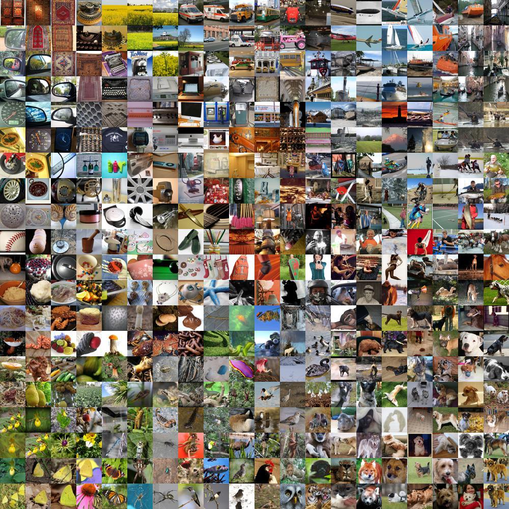
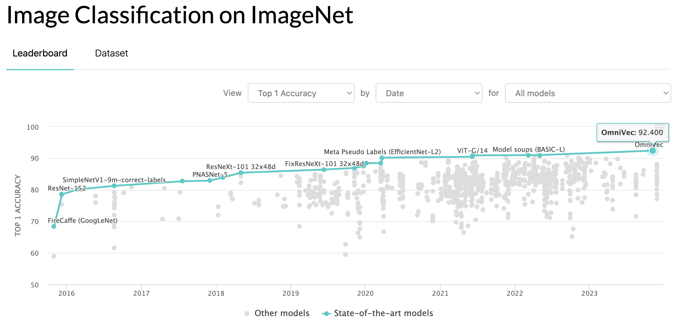
ImageNet

Open source repo of images consisting of more than 20K classes of over 14 million images (growing over the years).
AI researcher Fei-Fei Li began working on the idea for ImageNet in 2006.
Used as a benchmarking dataset in Computer Vision research.

AlexNet

AlexNet in 2012 was a game-changer (significance: GPU computation, also see Ilya Sutskever)
AlexNet consists of eight layers, with five convolutional layers and three fully connected layers (including the output layer).
The convolutional layers are followed by max-pooling layers
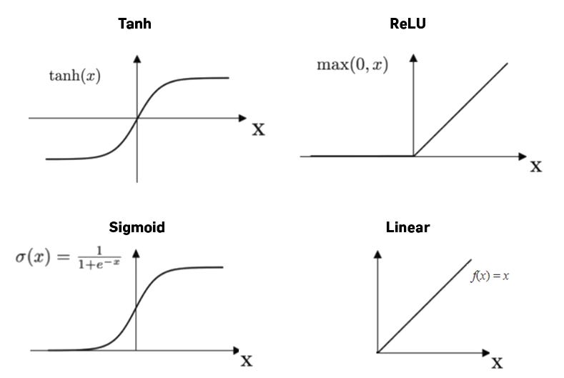
ReLU activation functions are used throughout the network to introduce non-linearity.

import torch
import torch.nn as nn
import torch.optim as optim
import torchvision
import torchvision.transforms as transforms
from torchvision.models import alexnet

import matplotlib.pyplot as plt
import numpy as np
import time

transform = transforms.Compose([
    transforms.Resize(256),
    transforms.CenterCrop(224),
    transforms.ToTensor(),
    transforms.Normalize((0.5, 0.5, 0.5), (0.5, 0.5, 0.5))
])

device = torch.device("cuda" if torch.cuda.is_available() else "cpu")
device

device(type='cuda')

trainset = torchvision.datasets.CIFAR10(root='./data', train=True, download=True, transform=transform)
trainloader = torch.utils.data.DataLoader(trainset, batch_size=4, shuffle=True, num_workers=2)

testset = torchvision.datasets.CIFAR10(root='./data', train=False, download=True, transform=transform)
testloader = torch.utils.data.DataLoader(testset, batch_size=4, shuffle=False, num_workers=2)

Files already downloaded and verified
Files already downloaded and verified

classes = ('Airplane', 'Car', 'Bird', 'Cat', 'Deer', 'Dog', 'Frog', 'Horse', 'Ship', 'Truck')

def imshow(img):
    img = img / 2 + 0.5
    npimg = img.numpy()
    plt.imshow(np.transpose(npimg, (1, 2, 0)))
    plt.show()

dataiter = iter(trainloader)
images, labels = next(dataiter)

imshow(torchvision.utils.make_grid(images))
print(' '.join('%5s' % classes[labels[j]] for j in range(4)))

png

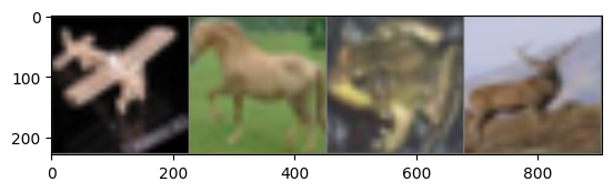
Airplane Horse  Frog  Deer

class AlexNet(nn.Module):
    def __init__(self):
        super(AlexNet, self).__init__()
        self.features = alexnet(pretrained=False).features
        self.avgpool = nn.AdaptiveAvgPool2d((6, 6))
        self.classifier = nn.Sequential(
            nn.Dropout(),
            nn.Linear(256 * 6 * 6, 4096),
            nn.ReLU(inplace=True),
            nn.Dropout(),
            nn.Linear(4096, 4096),
            nn.ReLU(inplace=True),
            nn.Linear(4096, 10),
        )

    def forward(self, x):
        x = self.features(x)
        x = self.avgpool(x)
        x = torch.flatten(x, 1)
        x = self.classifier(x)
        return x


alexnet_model = AlexNet().to(device)

criterion = nn.CrossEntropyLoss()
optimizer = optim.SGD(alexnet_model.parameters(), lr=0.001, momentum=0.9)


for epoch in range(5):
    running_loss = 0.0
    for i, data in enumerate(trainloader, 0):
        inputs, labels = data[0].to(device), data[1].to(device)
        optimizer.zero_grad()
        outputs = alexnet_model(inputs)
        loss = criterion(outputs, labels)
        loss.backward()
        optimizer.step()

        running_loss += loss.item()
        if i % 2000 == 1999:
            print(f"[{epoch + 1}, {i + 1}] loss: {running_loss / 2000:.3f}")
            running_loss = 0.0

print("Finished Training")

correct = 0
total = 0
with torch.no_grad():
    for data in testloader:
        images, labels = data[0].to(device), data[1].to(device)
        outputs = alexnet_model(images)
        _, predicted = torch.max(outputs.data, 1)
        total += labels.size(0)
        correct += (predicted == labels).sum().item()

print(f"Accuracy of the network on the 10000 test images: {100 * correct / total}%")

[1, 2000] loss: 2.298
[1, 4000] loss: 2.061
[1, 6000] loss: 1.785
[1, 8000] loss: 1.635
[1, 10000] loss: 1.533
[1, 12000] loss: 1.452
[2, 2000] loss: 1.339
[2, 4000] loss: 1.262
[2, 6000] loss: 1.204
[2, 8000] loss: 1.150
[2, 10000] loss: 1.101
[2, 12000] loss: 1.061
[3, 2000] loss: 0.948
[3, 4000] loss: 0.950
[3, 6000] loss: 0.918
[3, 8000] loss: 0.889
[3, 10000] loss: 0.891
[3, 12000] loss: 0.878
[4, 2000] loss: 0.755
[4, 4000] loss: 0.785
[4, 6000] loss: 0.761
[4, 8000] loss: 0.752
[4, 10000] loss: 0.752
[4, 12000] loss: 0.732
[5, 2000] loss: 0.626
[5, 4000] loss: 0.653
[5, 6000] loss: 0.643
[5, 8000] loss: 0.644
[5, 10000] loss: 0.637
[5, 12000] loss: 0.651
Finished Training
Accuracy of the network on the 10000 test images: 76.56%

ResNet

class ResNet(nn.Module):
    def __init__(self):
        super(ResNet, self).__init__()
        resnet_model = models.resnet18(pretrained=False) 
        self.features = nn.Sequential(*list(resnet_model.children())[:-1]) 
        self.avgpool = nn.AdaptiveAvgPool2d((1, 1))
        self.classifier = nn.Linear(resnet_model.fc.in_features, 10) 

    def forward(self, x):
        x = self.features(x)
        x = self.avgpool(x)
        x = x.view(x.size(0), -1)
        x = self.classifier(x)
        return x

resnet_model = ResNet().to(device)

criterion = nn.CrossEntropyLoss()
optimizer = optim.SGD(resnet_model.parameters(), lr=0.001, momentum=0.9)

for epoch in range(5):
    running_loss = 0.0
    for i, data in enumerate(trainloader, 0):
        inputs, labels = data[0].to(device), data[1].to(device)
        optimizer.zero_grad()
        outputs = resnet_model(inputs)
        loss = criterion(outputs, labels)
        loss.backward()
        optimizer.step()

        running_loss += loss.item()
        if i % 2000 == 1999:
            print(f"[{epoch + 1}, {i + 1}] loss: {running_loss / 2000:.3f}")
            running_loss = 0.0

print("Finished Training")

correct = 0
total = 0
with torch.no_grad():
    for data in testloader:
        images, labels = data[0].to(device), data[1].to(device)
        outputs = resnet_model(images)
        _, predicted = torch.max(outputs.data, 1)
        total += labels.size(0)
        correct += (predicted == labels).sum().item()

print(f"Accuracy of the network on the 10000 test images: {100 * correct / total}%")

[1, 2000] loss: 2.086
[1, 4000] loss: 1.792
[1, 6000] loss: 1.675
[1, 8000] loss: 1.485
[1, 10000] loss: 1.356
[1, 12000] loss: 1.252
[2, 2000] loss: 1.136
[2, 4000] loss: 1.101
[2, 6000] loss: 1.029
[2, 8000] loss: 0.981
[2, 10000] loss: 0.948
[2, 12000] loss: 0.891
[3, 2000] loss: 0.787
[3, 4000] loss: 0.793
[3, 6000] loss: 0.756
[3, 8000] loss: 0.747
[3, 10000] loss: 0.724
[3, 12000] loss: 0.724
[4, 2000] loss: 0.619
[4, 4000] loss: 0.620
[4, 6000] loss: 0.616
[4, 8000] loss: 0.595
[4, 10000] loss: 0.615
[4, 12000] loss: 0.568
[5, 2000] loss: 0.481
[5, 4000] loss: 0.503
[5, 6000] loss: 0.494
[5, 8000] loss: 0.510
[5, 10000] loss: 0.498
[5, 12000] loss: 0.502
Finished Training
Accuracy of the network on the 10000 test images: 80.16%

SOTA

SOTA is an acronym for State-Of-The-Art
the best models that can be used for achieving the results in a specific task (may be for a specific dataset as well)

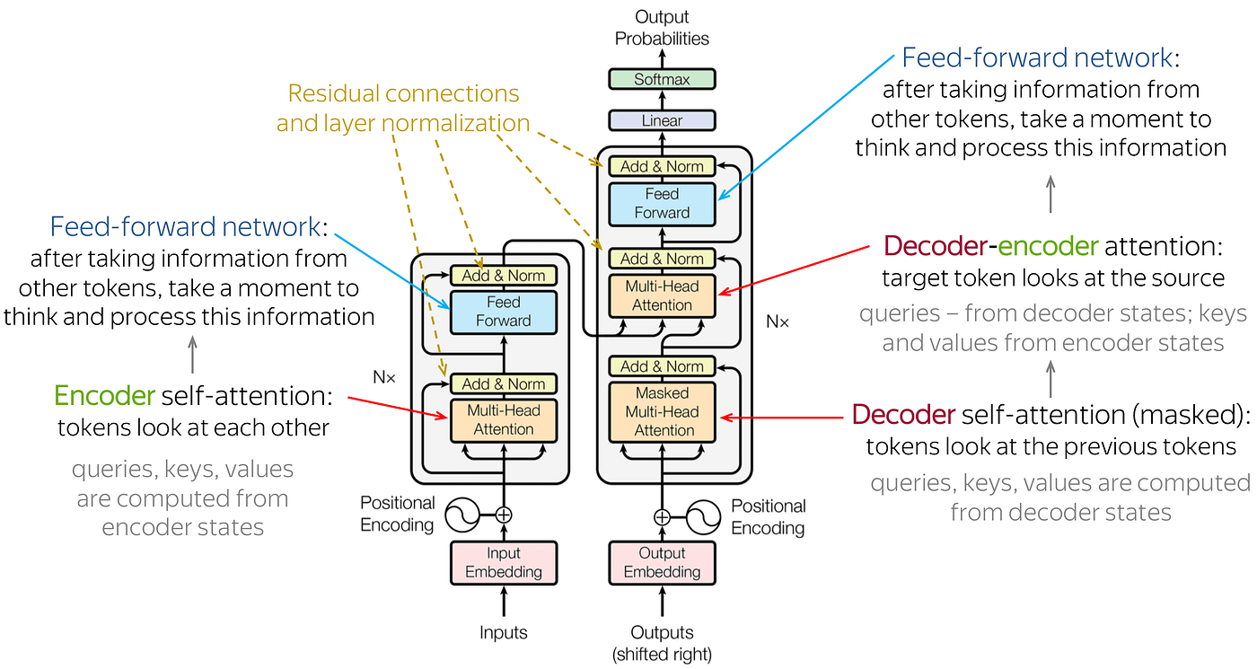
Transformer Architecture

Embeddings are representations of words or tokens in a continuous vector space. Each word/token in a sequence is mapped to a high-dimensional vector. In the Transformer model, embeddings are used to represent the input tokens. These embeddings serve as the initial input to the model, and they capture the semantic information of the tokens.

Attention mechanisms allow a model to focus on different parts of the input sequence when making predictions. It assigns different weights to different elements of the sequence. The Transformer uses a self-attention mechanism, which means that each element in the sequence can attend to all other elements. This allows the model to weigh the importance of different words in the context of the entire sequence.

In the Transformer model, the self-attention mechanism is applied to the input embeddings. Each element in the sequence (word embedding) can attend to all other elements, capturing dependencies and relationships between words. The attention mechanism assigns weights to each element based on its relevance to the others. These weights are used to compute a weighted sum of the input embeddings. This weighted sum is a context vector that represents the importance of different parts of the input sequence for the current position.

Since Transformer models do not inherently capture the order of elements in a sequence, positional encoding is added to the input embeddings to provide information about the position of each token. Positional encoding ensures that the model understands the sequential order of the input tokens, allowing it to process sequences effectively.

The Transformer architecture consists of an encoder and a decoder. Each encoder layer contains a multi-head self-attention mechanism and a feedforward neural network. The attention mechanism in the encoder captures relationships between different words in the input sequence. The embeddings, enriched by attention, flow through the layers of the encoder, allowing the model to learn complex patterns and dependencies.

Core Idea of the Paper

The paper introduces the use of Transformers, originally designed for natural language processing, in image recognition tasks.
Transformers are known for their success in processing sequential data, and the paper aims to leverage their capabilities for image understanding.
The authors propose treating an image as a sequence of fixed-size patches, each represented as a vector, to make it compatible with the sequential nature of Transformers.
The image patches are linearly embedded to create token representations, which serve as input to the Transformer model.
The architecture involves a stack of Transformer layers, allowing the model to capture global and local relationships within the image.
To maintain spatial information, positional encoding is added to the patch embeddings, enabling the model to understand the arrangement of patches in the image.
The model is trained on large-scale datasets, emphasizing the importance of data size in achieving superior performance in image recognition.
The paper compares the performance of Transformer models with convolutional neural networks (CNNs) on image classification tasks.
Transformers are shown to be highly scalable, allowing efficient processing of large images and achieving state-of-the-art results on various benchmarks.
The study demonstrates the transferability of pre-trained Transformer models to different downstream tasks, showcasing their versatility and effectiveness in diverse image recognition applications.

Colab Walkthrough

Ayush Subedi

[Paper Exploration] An Image is Worth 16x16 Words: Transformers for Image Recognition at Scale

An Image is Worth 16x16 Words: Transformers for Image Recognition at Scale: An exploration on how ViT can be used for vision.