General overview and key concepts

In plain English, optimization is the action of making the best or most effective use of a situation or resource. Optimization problems are of great practical interest. For example, in manufacturing, how should one cut plates of a material so that the waste is minimized? In business, how should a company allocate the available resources that its profit is maximized? Some of the first optimization problems have been solved in ancient Greece and are regarded among the most significant discoveries of that time. In the first century A.D., the Alexandrian mathematician Heron solved the problem of finding the shortest path between two points by way of the mirror.

This result, also known as Heron’s theorem of the light ray, can be viewed as the origin of the theory of geometrical optics. The problem of finding extreme values gained special importance in the seventeenth century, when it served as one of the motivations in the invention of differential calculus, which is the foundation of the modern theory of mathematical optimization.

Generic form of optimization problem:

$min$ $f(x)$ $s.t.$ $x \in X $

• The vector $x = (x_1, . . . , x_n)$ is the optimization variable (or decision variable) of the problem
• The function $f$ is the objective function
• A vector $x$ is called optimal, or a solution (not optimal solution) of the problem, if it has the smallest objective value among all vectors that satisfy the constraints
• $X$ is the set of inequality constraints

Mathematical ingredients:

• Encode decisions/actions as decision variables whose values we are seeking
• Identify the relevant problem data
• Express constraints on the values of the decision variables as mathematical relationships (inequalities) between the variables and problem data
• Express the objective function as a function of the decision variables and the problem data.

Minimize or Maximize an objective function of decision variable subject to constraints on the values of the decision variables.

min or max f(x1, x2, .... , xn)
subject to gi(x1, x2, ...., ) <= bi     i = 1,....,m 
        xj is continuous or discrete    j = 1,....,n

The problem setting

• Finite number of decision variables
• A single objective function of decision variables and problem data
  • Multiple objective functions are handled by either taking a weighted combination of them or by optimizing one of the objectives while ensuring the other objectives meet target requirements.
• The constraints are defined by a finite number of inequalities or equalities involving functions of the decision variables and problem data
• There may be domain restrictions (continuous or discrete) on some of the variables
• The functions defining the objective and constraints are algebraic (typically with rational coefficients)

Minimization vs Maximization

• Without the loss of generality, it is sufficient to consider a minimization objective since maximization of objective function is minimization of the negation of the objective function

Program vs Optimization

• A program or mathematical program is an optimization problem with a finite number of variables and constraints written out using explicit mathematical (algebraic) expressions
• The word program means plan/planning
• Early application of optimization arose in planning resource allocations and gave rise to programming to mean optimization (predates computer programming)

Example: Designing a box:

Given a $1$ feet by $1$ feet piece of cardboard, cut out corners and fold to make a box of maximum volume:
Decision: $x$ = how much to cut from each of the corners?
Alternatives: $0<=x<=1/2$
Best: Maximize volume: $V(x) = x(1-2x)^2$ ($x$ is the height and $(1-2x)^2$ is the base, and their product is the volume)
Optimization formulation: $max$ $x(1-2x)^2$ subject to $0<=x<=1/2$ (which are the constraints in this case)

This is an unconstrained optimization problem since the constraint is a simple bound based.

Example: Data Fitting:

Given $N$ data points $(y_1, x_1)…(y_N, x_N)$ where $y_i$ belongs to $\mathbb{R}$ and $x_i$ belongs to $\mathbb{R}^n$, for all $i = 1..N$, find a line $y = a^Tx+b$ that best fits the data.
Decision: A vector $a$ that belongs to $\mathbb{R}^n$ and a scalar $b$ that belongs to $\mathbb{R}$
Alternatives: All $n$-dimensional vectors and scalars
Best: Minimize the sum of squared errors
Optimization formulation: $\begin{array}{ll}\min & \sum_{i=1}^N\left(y_i-a^{\top} x_i-b\right)^2 \ \text { s.t. } & a \in \mathbb{R}^n, b \in \mathbb{R}\end{array}$

This is also an unconstrained optimization problem.

Example: Product Mix:

A firm make $n$ different products using $m$ types of resources. Each unit of product $i$ generates $p_i$ dollars of profit, and requires $r_{ij}$ units of resource $j$. The firm has $u_j$ units of resource $j$ available. How much of each product should the firm make to maximize profits?
Decision: how much of each product to make
Alternatives: defined by the resource limits
Best: Maximize profits
Optimization formulation:
Sum notation: $\begin{array}{lll}\max & \sum_{i=1}^n p_i x_i \ \text { s.t. } & \sum_{i=1}^n r_{i j} x_i \leq u_j & \forall j=1, \ldots, m \ & x_i \geq 0 & \forall i=1, \ldots, n\end{array}$
Matrix notation: $\begin{array}{cl}\max & p^{\top} x \ \text { s.t. } & R x \leq u \ & x \geq 0\end{array}$

Example: Project investment

A firm is considering investing in $n$ different R&D projects. Project $j$ requires an investment of $c_j$ dollars and promises a return of $r_j$ dollars. The firm has a budget of $B$ dollars. Which projects should the firm invest in?
Decision: Whether or not to invest in project
Alternatives: Defined by budget
Best: Maximize return on investment
Sum notation: $\begin{aligned} \max & \sum_{j=1}^n r_j x_j \ \text { s.t. } & \sum_{j=1}^n c_j x_j \leq B \ & x_j \in{0,1} \forall j=1, \ldots, n\end{aligned}$
Matrix notation: $\begin{aligned} \max & r^{\top} x \ \text { s.t. } & c^{\top} x \leq B \ & x \in{0,1}^n\end{aligned}$

This is not an unconstrained problem.

• Identify basic portfolio optimization and associated issues
• Examine the Markowitz Portfolio Optimization approach
  • Markowitz Principle: Select a portfolio that attempts to maximize the expected return and minimize the variance of returns (risk)
• For multi objective problem (like defined by the Markowitz Principle), two objectives can be combined:
  • Maximize Expected Return - $\lambda$*risk
  • Maximize Expected Return subject to risk <= s_max (constraint on risk)
  • Minimize Risk subject to return >= r_min (threshold on expected returns)
• Optimization Problem Statement

Given $1000, how much should we invest in each of the three stocks MSFT, V and WMT so as to :
- have a one month expected return of at least a given threshold
- minimize the risk(variance) of the portfolio return

• Decision: investment in each stock
• alternatives: any investment that meets the budget and the minimum expected return requirement
• best: minimize variance
• Key trade-off: How much of the detail of the actual problem to consider while maintaining computational tractability of the mathematical model?
• Requires making simplifying assumptions, either because some of the problem characteristics are not well-defined mathematically, or because we wish to develop a model that can actually be solved
• Need to exercise great caution in these assumptions and not loose sight of the true underlying problem
• Assumptions:
  • No transaction cost
  • Stocks does not need to be bought in blocks (any amount >=0 is fine)
• Optimization Process: Decision Problem -> Model -> Data Collection -> Model Solution -> Analysis -> Problem solution
• No clear cut recipe
• Lots of feedbacks and iterations
• Approximations and assumptions involved in each stage
• Success requires good understanding of the actual problem (domain knowledge is important)

Classification of optimization problems

• The tractability of a large scale optimization problem depends on the structure of the functions that make up the objective and constraints, and the domain restrictions on the variables.

Functions	Variable domains	Problem Type	Difficulty
All linear	Continuous variables	Linear Program	Easy
Some nonlinear	Continuous variables	Nonlinear Program or Nonlinear Optimization Problem	Easy/Difficult
Linear/nonlinear	Some discrete	Integer Problem or Discrete Optimization Problem	Difficult

Optimization Problem	Description	Difficulty
Linear Programming	A linear programming problem involves maximizing or minimizing a linear objective function subject to a set of linear constraints	Easy to moderate
Nonlinear Programming	A nonlinear programming problem involves optimizing a function that is not linear, subject to a set of nonlinear constraints	Moderate to hard
Quadratic Programming	A quadratic programming problem involves optimizing a quadratic objective function subject to a set of linear constraints	Moderate
Convex Optimization	A convex optimization problem involves optimizing a convex function subject to a set of linear or convex constraints	Easy to moderate
Integer Programming	An integer programming problem involves optimizing a linear or nonlinear objective function subject to a set of linear or nonlinear constraints, where some or all of the variables are restricted to integer values	Hard
Mixed-integer Programming	A mixed-integer programming problem is a generalization of integer programming where some or all of the variables can be restricted to integer values or continuous values	Hard
Global Optimization	A global optimization problem involves finding the global optimum of a function subject to a set of constraints, which may be nonlinear or non-convex	Hard
Stochastic Optimization	A stochastic optimization problem involves optimizing an objective function that depends on random variables, subject to a set of constraints	Hard

Subclasses of NLP (Non Linear Problem)

• Unconstrained optimization: No constraints or simple bound constraints on the variables (Box design example above)
• Quadratic programming: Objectives and constraints involve quadratic functions (Data fitting example above), subset of NLP

Subclasses of IP (Integer Programming)

• Mixed Integer Linear Program
  • All linear functions
  • Some variables are continuous and some are discrete
• Mixed Integer Nonlinear Program (MINLP)
  • Some nonlinear functions
  • Some variables are continuous and some are discrete
• Mixed Integer Quadratic Program (MIQLP)
  • Nonlinear functions are quadratic
  • Some variables are continuous and some are discrete
  • subset of MINLP

Why and how to classify?

• Important to recognize the type of an optimization problem:
  • to formulate problems to be amenable to certain solution methods
  • to anticipate the difficulty of solving the problem
  • to know which solution methods to use
  • to design customized solution methods
• how to classify:
  • check domain restriction on variables
  • check the structure of the functions involved

Linear Algebra Primer

• Vectors: Vectors are mathematical objects that have both magnitude and direction. They can be represented as ordered lists of numbers or as arrows in space. Vectors are often used to represent physical quantities such as velocity or force. In two-dimensional space, a vector is represented by an ordered pair of numbers (x, y), and in three-dimensional space, it is represented by an ordered triple (x, y, z). Vectors can be added and subtracted, and multiplied by a scalar (a single number). They also have properties such as the dot product and cross product. In computer science and programming, a vector is also a data structure that can store multiple values of the same type.
• Matrices: Matrices are rectangular arrays of numbers that can be used to represent linear transformations and systems of linear equations. They are also used to represent data in statistics and machine learning.
• Linear equations: Linear equations are equations that involve only linear terms, such as x and y, rather than more complex functions like sin(x) or e^x. They can be represented using matrices and solved using techniques like Gaussian elimination.
• Eigenvectors and eigenvalues: Eigenvectors are special vectors that are unchanged by a linear transformation, except for a scaling factor. Eigenvalues are the corresponding scaling factors. They are useful in many applications, such as analyzing networks and modeling physical systems.
• Vector spaces: Vector spaces are sets of vectors that satisfy certain properties, such as closure under addition and scalar multiplication. They are used to represent many mathematical objects, such as functions and polynomials.
• Inner products: An inner product is a function that takes two vectors as input and produces a scalar as output. It is used to measure the angle between vectors and the length of a vector.
• Orthogonality: Two vectors are orthogonal if they are perpendicular to each other. Orthogonal vectors have many important applications, such as in least squares regression and in the Gram-Schmidt process for orthonormalizing a set of vectors.
• The second derivative test is a method used in calculus to determine the nature of the critical points of a function, which can be either a maximum, minimum, or saddle point.
• A critical point is a point on the graph of a function where the derivative is either zero or undefined.
• To apply the second derivative test, we need to find the critical points of the function by setting its first derivative equal to zero and solving for the variables. Then, we can determine the nature of these critical points by examining the sign of the second derivative of the function evaluated at the critical points. Specifically:
  • If the second derivative is positive at a critical point, then the function has a local minimum at that point.
  • If the second derivative is negative at a critical point, then the function has a local maximum at that point.
  • If the second derivative is zero at a critical point, then the second derivative test is inconclusive, and we need to use other methods to determine the nature of the critical point.
• The vectors $x$ and $y$ are orthogonal if $x^Ty=0$, they make an acute angle if $x^Ty>0$ and an obtuse angle if $x^Ty<0$
• Also, $x^Ty=||x||.||y||cos\theta$
• A set of vectors are linearly independent if none of the vectors can be written as a linear combination of the others. That is the unique solution to the system of equations. There can be at most $n$ linearly independent vectors in $R^n$
• Any collection of $n$ linearly independent vectors in $R$ defines a basis (or a coordinate system) of $R^n$, any vector in $R^n$ can be written as a linear combination of the basis vectors The unit vectors $e^1= [1, 0, …0]^T$, $e^2= [0, 1, …0]^T$,…,$e^n= [0, 0, …1]^T$, define the standard basis for $R^n$
• The rank of a matrix is a measure of the “nondegeneracy” of the matrix and it is one of the most important concepts in linear algebra. It is defined as the dimension of the vector space spanned by its columns or rows. Intuitively, it represents the number of linearly independent columns or rows in the matrix.
• row rank = column rank = rank($A$). $A$ is full rank if rank($A$) = min($m$, $n$)
• A system of equations has a solution when the equations are consistent, meaning that there is at least one set of values for the variables that satisfies all of the equations. If the equations are inconsistent, meaning that there is no set of values that satisfies all of the equations, then the system of equations has no solution.
• An affine function is a function that is defined as a linear combination of variables, with the addition of a constant term. An affine function can be written as:

f(x) = a_1x_1 + a_2x_2 + ... + a_nx_n + b

Where x_1, x_2, …, x_n are the input variables, a_1, a_2, …, a_n are the coefficients, and b is a constant term. An affine function is a generalization of a linear function, which does not have the constant term.

Multivariate Calculus Primer

Hessian matrix

• The Hessian matrix is a square matrix of second-order partial derivatives of a scalar-valued function of multiple variables.
• The Hessian matrix of a scalar-valued function f(x) of n variables x = (x1, x2, …, xn) is defined as the matrix of second-order partial derivatives of f with respect to x, with the i-th row and j-th column containing the second partial derivative of f with respect to xi and xj.
• The Hessian matrix is often used in optimization, for example, to find the local minima or maxima of a function. A point where the Hessian is positive definite is a local minimum, while a point where the Hessian is negative definite is a local maximum. If the Hessian is positive semi-definite, it’s a saddle point.
• It is important to notice that the Hessian Matrix is symmetric, therefore it has real eigenvalues and it is diagonalisable.
• $H(f)_{i,j}=\frac{\partial^2f}{\partial x_i \partial x_j}$
• The symmetry of second derivatives (also called the equality of mixed partials) refers to the possibility of interchanging the order of taking partial derivatives of a function. The symmetry is the assertion that the second-order partial derivatives satisfy the identity. In the context of partial differential equations it is called the Schwarz integrability condition.
• $\frac{\partial^2f}{\partial x_i \partial x_j} = \frac{\partial^2f}{\partial x_j \partial x_i}$

Taylor Approximation

The Taylor series of a real or complex-valued function f (x) that is infinitely differentiable at a real or complex number a is the power series.

Let $f: \mathbb{R}^n \rightarrow \mathbb{R}$ be a differentiable function and $\mathbf{x}^0 \in \mathbb{R}^n$.

• First order Taylor’s approximation of $f$ at $\mathbf{x}^0$ : $$ f(\mathbf{x}) \approx f\left(\mathbf{x}^0\right)+\nabla f\left(\mathbf{x}^0\right)^{\top}\left(\mathbf{x}-\mathbf{x}^0\right) $$
• Second order Taylor’s approximation of $f$ at $\mathbf{x}^0$ : $$ f(\mathbf{x}) \approx f\left(\mathbf{x}^0\right)+\nabla f\left(\mathbf{x}^0\right)^{\top}\left(\mathbf{x}-\mathbf{x}^0\right)+\frac{1}{2}\left(\mathbf{x}-\mathbf{x}^0\right)^{\top} \nabla^2 f\left(\mathbf{x}^0\right)\left(\mathbf{x}-\mathbf{x}^0\right) $$ `

Sets in Optimization Problems

• A set is closed if it includes its boundary points.
• Intersection of closed sets is closed.
• Typically, if none of inequalities are strict, then the set is closed.
• A set is convex if a line segment connecting two points in the set lies entirely in the set.
• A set is bounded if it can be enclosed in a large enough (hyper)-sphere or a box.
• A set that is both bounded and closed is called compact.
  • $R^2$ is closed but not bounded
  • $x^2+y^2<1$ is bounded but not closed
  • $x+y>=1$ is closed but not bounded
  • $x^2+y^2<=1$ is closed and bounded (compact)
• An optimal solution of maximizing a convex function over a compact set lies on the boundary of the set.

Convex Function

• A function $f: \mathbb{R}^n \rightarrow \mathbb{R}$ is convex if $$ f(\lambda \mathbf{x}+(1-\lambda) \mathbf{y}) \leq \lambda f(\mathbf{x})+(1-\lambda) f(\mathbf{y}) \quad \forall \mathbf{x}, \mathbf{y} \in \mathbb{R}^n \text { and } \lambda \in[0,1] $$
• “Function value at the average is less than the average of the function values”
• This also implies that $a^Tx+b$ is convex (and concave)
• For a convex function the first order Taylor’s approximation is a global under estimator
• A convex optimization problem has a convex objective and convex set of solutions.
• Linear programs (LPs) can be seen as a special case of convex optimization problems. In an LP, the objective function and constraints are linear, which means that the feasible region defined by the constraints is a convex set. As a result, the optimal solution to an LP is guaranteed to be at a vertex (corner) of the feasible region, which makes it a convex optimization problem.
• A twice differentiable univariate function is convex if $f^{’’}(x)>=0$ for all $x \in R$
• To generalize, a twice differentiable function is convex if and only if the Hessian matrix is positive semi definite.
• A positive semi-definite (PSD) matrix is a matrix that is symmetric and has non-negative eigenvalues. In the context of a Hessian matrix, it represents the second-order partial derivatives of a multivariate function and reflects the curvature of the function. If the Hessian is PSD, it indicates that the function is locally convex, meaning that it has a minimum value in the vicinity of that point. On the other hand, if the Hessian is not PSD, the function may have a saddle point or be locally non-convex. The PSD property of a Hessian matrix is important in optimization, as it guarantees the existence of a minimum value for the function.
• Sylvester’s criterion is a method for determining if a matrix is positive definite or positive semi-definite. The criterion states that a real symmetric matrix is positive definite if and only if all of its leading principal minors (i.e. determinants of the submatrices formed by taking the first few rows and columns of the matrix) are positive. If all the leading principal minors are non-negative, then the matrix is positive semi-definite.

Operations preserving convexity

• Nonnegative weighted sum of convex functions is convex, i.e. if $f_i$ is convex and $\alpha_i \geq 0$ for all $i=1, \ldots, m$, then $g(\mathbf{x})=\sum_{i=1}^m \alpha_i f_i(\mathbf{x})$ is convex.
• Maximum of convex functions is convex.
• Composition: Let $f: \mathbb{R}^m \rightarrow \mathbb{R}$ be a convex function, and $g_i: \mathbb{R}^n \rightarrow \mathbb{R}$ be convex for all $i=1, \ldots, m$. Then the composite function $$ h(\mathbf{x})=f\left(g_1(\mathbf{x}), g_2(\mathbf{x}), \ldots, g_m(\mathbf{x})\right) $$ is convex if either $f$ is nondecreasing or if each $q_i$ is a linear function.

Convexity Preserving Set Operations

• Intersection of convex sets is a convex set
• Intersection of non convex sets might be a convex set
• Union of two convex set might not be a convex set
• Sum of convex set is a convex set
• Product of convex set is a convex set

Convex Optimization Problem

• An optimization problem (in minimization) form is a convex optimization problem, if the objective function is a convex function and constraint set is a convex set.
• The problem $min$ ${f(x) : x \in X}$ is a convex optimization problem if $f$ is a convex function and $X$ is a convex set.
• To check if a given problem is convex, we can check convexity of each constraint separately. (This is a sufficient test, not necessary).
• $\begin{array}{cl}\min & f(\mathbf{x}) \ \text { s.t. } \end{array}$ $\begin{array}{cl} g_i(\mathbf{x}) \leq b_i \quad i=1, \ldots, m \ & h_j(\mathbf{x})=d_j \quad j=1, \ldots, \ell \ & \mathbf{x} \in \mathbb{R}^n\end{array}$

Sufficient and necessary

• In mathematical logic, the terms “sufficient” and “necessary” are used to describe the relationship between two conditions.
• A condition A is considered “sufficient” for a condition B if whenever condition A is true, condition B is also guaranteed to be true. In other words, if A is sufficient for B, then having A implies having B.
• A condition B is considered “necessary” for a condition A if whenever condition B is false, condition A is also guaranteed to be false. In other words, if B is necessary for A, then not having B implies not having A.
• Together, “necessary and sufficient” means that the two conditions are equivalent, in the sense that if one is true, then the other must also be true, and if one is false, then the other must also be false. In mathematical terms, A is necessary and sufficient for B if and only if (A if and only if B).
• “being a male is a necessary condition for being a brother, but it is not sufficient — while being a male sibling is a necessary and sufficient condition for being a brother”

Epigraph of a function

• An epigraph of a function is a graphical representation of the function’s domain and range. It is formed by the region above the graph of the function and the line x = a for some value of a. The epigraph represents all possible values of the function for all values of x greater than or equal to a. It is used in optimization problems to visualize the feasible region for the optimization variable.
• A function (in black) is convex if and only if the region above its graph (in green) is a convex set. This region is the function’s epigraph.
• The epigraph and the $\alpha$ level set, of a convex function are convex sets.

Outcomes of Optimization

• Any $x \in X$ is a feasible solution of the optimization problem (P)
• Feasible solution = A solution that satisfies all the constraints
• An unbounded problem must be feasible
• An optimization problem is unbounded, if there are feasible solutions with arbitrarily small objective values.(limits to negative infinity for minimization problem)
• If $X=\emptyset$ then no feasible solutions exist, and the problem (P) is said to be infeasible.
• If $X$ is a bounded set, then P cannot be unbounded
• The problem $\min {3x+ 2y: x+ y<=1,x>=2,y>=2}$ is infeasible
• An optimization problem can have 4 possible outcomes. The outcome can be infeasible, unbounded (but feasible), have no optimal solution, have one optimal solution, or have multiple optimal solutions

Existence of Optimal Solutions

• The Weierstrass extreme value theorem asserts that if you minimize a continuous function over a closed and bounded set in $R_n$, then the minimum will be achieved at some point in the set.
• Sufficient conditions: if the constraint set is bounded and non empty (feasible), then continuity and closedness guarantees an optimal solution exist.

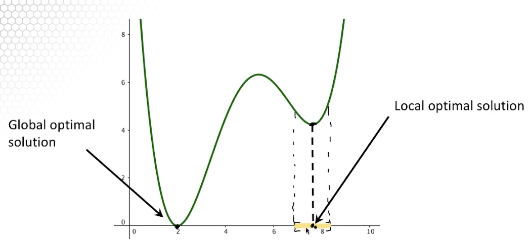
Local and Global Optimal Solutions

• Local optimal solutions are also global optimal solutions for convex optimization problems
• Every global optimal solution is a local optimal solution, but not vice versa
• The objective function value at different local optimal solutions may be different
• The objective function value at all global solutions must be the same
• If the problem is convex, since any local solution is a global solution, we can be sure that if we find a local solution, that is also a global solution.

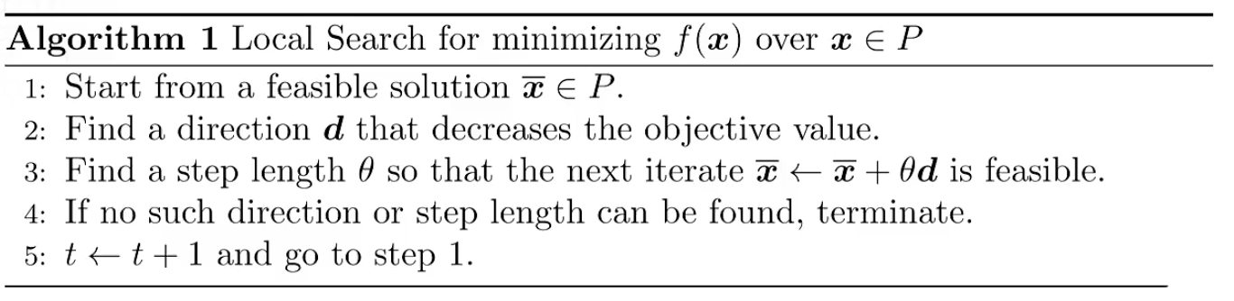
Idea of Improving Search

• Most optimization algorithms are based on the paradigm of improving search:
  • Start from a feasible solution
  • Move to a new feasible solution with a better objective value, Stop if not possible
  • Repeat step 2
• In general, we are only able to look in the “neighborhood” of the current solution in search of a better feasible solution (solutions that are within a small positive distance from the current solution)
• The move direction and step size should ensure that the new point is feasible and has an improved objective function value
• The improving search is better for local solutions, but for convex, in principal it can be used to find global solutions (by definition)

Optimality Certificates

Optimality Certificates and Relaxations

• A certificate or a stopping condition is an easily checkable condition such that if the current solution satisfies this condition then it is guaranteed to be optimal or near optimal
• Lower bound (a Priori) that the objective value of any solution cannot be lower than.
• Suppose we have a feasible solution $x’$ to an optimization problem with an objective value of $f(x’)$. Suppose the optimal objective value of the problem is $v*$. Then the absolute optimality gap of the solution is $gap(x’)$ = $f(x’) - v*$. And, the relative gap is $(f(x’) - v*)$/$v*$. The gap and rgap are always non negative.
• We do not know $v*$ but we do know the lower bound $L$. From definition, $L<=v*<=f(x’)$
• A lower bound allows us to get an upper bound on the solution.
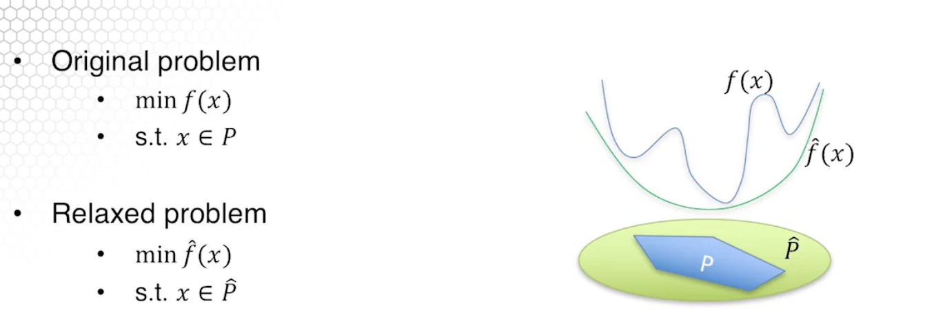
• For two optimization problem (P) $min$ $f(x)$ $s.t.$ $x \in X $ and (Q) $min$ $g(x)$ $s.t.$ $x \in Y $, Problem (Q) is a relaxation of P
  • if $X \subseteq Y$ (problem Q admits more solution than P) and/or
  • $f(x) >= g(x) \forall x \in X $
• Obtained by enlarging the feasible region and underapproximating the objective function. We do not have to do both of those (see equals to sign)
• Relaxation should be easier to solve.
• Optimal value of the relaxation provides a lower bound on the original problem. (This provides the optimality certificate.)
• If the relaxation is infeasible then the original problem is also infeasible.
• Suppose only the constraints are relaxed, then if a solution to the relaxation is feasible to the original problem then it must be an optimal solution to the original problem.
• A lower bound on the optimal value provides a way to certify the quality of a given solution.

Lagrangian Relaxation and Duality

• Very specific type of relaxation
• Lagrangian relaxation is a method used in optimization to solve a difficult problem by relaxing some of its constraints and instead optimizing a modified objective function known as the Lagrangian function. The Lagrangian function is constructed by adding a penalty term for each constraint to the original objective function. The penalty term is multiplied by a non-negative Lagrange multiplier that represents the slack in the constraint. By choosing appropriate values for the multipliers, the relaxed problem can be made to approximate the original problem.
• The dual problem attempts to find the relaxation with the tightest bound (or the largest lower bound)
• Weak duality: dual optimal value <= original optimal value
• Some times we get strong duality (for LP)

Unconstrained Optimization: Derivative Based

Optimality Conditions

• Unconstrained, that is the constraints are only $x \in R^n$ and twice differentiable
• If a solution is a local optimal solution of an unconstrained problem, then the gradient vanishes at the point (First order optimality condition)
• Hessian is a positive semidefinite (Second order optimality condition)
• The conditions are necessary but not sufficient. Example: $f(x_$)$
• For example for, $f(x)=x^3$, at point 0, both of the conditions are satisfied. However, it is neither a local min or max.
• A sufficient (but not necessary) condition would be the gradient vanishing at the point, and is the Hessian is positive definite.

Gradient Descent

• The gradient descent method moves from one iteration to the next by moving along the negative of the gradient direction in order to minimize the function.
• Gradient descent is a optimization algorithm used to minimize the error of a machine learning model. It is an iterative method that updates the model parameters in the direction of the negative gradient of the cost function with respect to the parameters. The gradient indicates the direction of steepest increase in the cost function and the descent refers to moving in the direction of negative gradient to find the minimum of the cost function. The learning rate determines the size of the steps taken to reach the minimum and the algorithm stops when the change in cost is below a certain threshold or when a maximum number of iterations is reached.
• Let $x^k$ be the current iterate, and we want to chose a downhill direction $d^k$ and a step size $a$ such that $f(x^k+ad^k)<f(x^k)$
• By Taylor’s expansion, $f(x^k+ad^k) \approx f(x^k) + a \nabla f(x^k)^Td_k$
• So we want $\nabla f(x^k)^Td_k < 0$. The steepest descent direction is $d^k = - \nabla f(x^k) $
• Step size can be identified using a line search. That is, define a function $g(a) := f(x^k + ad^k)$. Choose $a$ to minimize $g$. It can also be a small fixed step size.

Newton’s Method

• Newton’s Method is a second-order optimization algorithm that is used to find the minimum of a function. It is an iterative method that updates the parameters by using the gradient of the function (first derivative) and the Hessian matrix (second derivative) to find the direction of the local minimum. The algorithm starts with an initial guess for the parameters and iteratively updates them using the Newton-Raphson formula until the change in the parameters is below a certain threshold or a maximum number of iterations is reached. Newton’s Method is faster and more precise than gradient descent for well-behaved functions, but it can be sensitive to poor initialization and can get stuck in local minima.
• $x^{k+1} $ = $x^k$ - $[\nabla^2$ $f(x_k)]^{-1}$ $ \nabla f(x^k)$
• If started close enough to local minimum and the Hessian is positive definite, then the method has quadratic convergence
• Not guaranteed to converge. The Newton direction may not be improving at all.
• If the Hessian is singular (or close to singular) at some iteration, we cannot proceed.
• Computing gradient as well as the Hessian and its inverse is expensive.

Quasi-Newton Methods

• Blend of gradient descent and Newton’s method.
• Avoids computation of Hessian and its inverse
• $x^{k+1} $ = $x^k$ - $a_k H_k$ $ \nabla f(x^k)$, where $H_k$ is an approximation of $[\nabla^2$ $f(x_k)]^{-1}$ and $a_k$ is determined by line search

Unconstrained Optimization: Derivative Free

Methods for Univariate Functions

• Golden Section Search: Start with an initial interval $[x_l, x_u]$ containing the minima, and successively narrow this interval
• Golden Section Search is an optimization algorithm used to find the minimum of a unimodal function, i.e., a function with a single minimum. The method is based on the idea of dividing an interval that contains the minimum into three sections, with the middle section being proportional to the golden ratio. The algorithm iteratively narrows down the interval by selecting the section that contains the minimum and discards the other sections. The process continues until the interval is sufficiently small and the minimum can be approximated with a desired accuracy. Golden Section Search is a bracketing method, which means it only requires the function to be unimodal and does not require the derivative or any other information about the function. It is a simple and efficient method for finding the minimum of unimodal functions, but it is slower than more sophisticated optimization methods for functions with multiple minima or more complex structures.
• Step 0: Set $x_1 = x_u - a(x_u-x_l)$ and $x_2=x_l+a(x_u-x_l)$
• Step 1: If $(x_u-x_l) <= \epsilon$ stop and return $x^* = 0.5(x_l+x_u)$ as the minima
• Example of how to use scipy.optimize.minimize to minimize a scalar function:

import numpy as np
from scipy.optimize import minimize

def objective_function(x):
    return x**2 + 5*np.sin(x)

x0 = np.array([1.0]) # Initial guess
result = minimize(objective_function, x0, method='BFGS')
print("Minimum at:", result.x)

Methods for Multivariate Function

• The Nelder-Mead method is a optimization algorithm used to minimize a scalar function of several variables. It is a derivative-free method, meaning that it does not require the gradient of the objective function to be calculated. It works by constructing a simplex (a set of vertices) in the high-dimensional space defined by the input variables, and then iteratively modifying the vertices to find the minimum.
• Here’s an example of how to use scipy.optimize.minimize with the Nelder-Mead method:

import numpy as np
from scipy.optimize import minimize

def objective_function(x):
    return x**2 + 5*np.sin(x)

x0 = np.array([1.0]) # Initial guess
result = minimize(objective_function, x0, method='Nelder-Mead')
print("Minimum at:", result.x)

• Nelder-Mead method is a numerical algorithm for minimizing a multivariate function using only function evaluations
• It is not guaranteed to converge but often works well.

Linear optimization

Linear Optimization Modeling - Network Flow Problems

Introduction to LP Modeling

• A linear program is composed of:
  • Variables $x=(x_1,x_2,x_3…,x_n)$
  • Linear objective function $f(x_1,x_2,x_3…,x_n)=\sum_{i=1}^n c_i x_i = c^Tx$
  • Linear constraints: $>=, <= or =$
• All linear problems can be written as a inner product of two vectors.
• The objective function must be a linear function of the variables.
• The constraints must be linear inequality or equality constraints.

Optimal Transportation Problem

• The transportation problem is a type of linear programming problem that deals with finding the optimal assignment of resources to meet a set of demands. The problem is typically framed as a network flow problem, where the goal is to find the maximum flow from a set of sources to a set of destinations.
• In a transportation problem, the goal is to find the least cost way to transport a given amount of goods from a set of sources (e.g. factories) to a set of destinations (e.g. warehouses) subject to certain constraints such as limited supply at the sources and limited demand at the destinations. The cost of transporting a unit of goods from a source to a destination is represented by a cost matrix, which is usually obtained through market research or historical data.
• There are various algorithms that can be used to solve transportation problems, including the North-West Corner Method, the Minimum Cost Method (also known as the Vogel’s Approximation Method), and the Modified Distribution Method. The most popular algorithm for solving transportation problems is the Iterative Proportional Fitting (IPF) algorithm, also known as the MODI (Modified Distribution) method.
• The transportation problem is an important optimization problem with numerous real-world applications, including supply chain management, distribution systems, and logistics planning.
• There are $m$ suppliers, $n$ customers. Supplier $i$ can supply up to $s_i$ units of supply, and customer $j$ has $d_j$ units of demand. It costs $c_{ij}$ to transport a unit of product from supplier $i$ to customer $j$. We want to find a transportation schedule to satisfy all the demand within minimum transportation cost.
• Formulation 1: $\begin{array}{ll}\min & \sum_{i=1}^m \sum_{j=1}^n c_{i j} x_{i j} \ \text { s.t. } & \sum_{i=1}^m x_{i j}=d_j, \quad \forall j \ & \sum_{j=1}^n x_{i j} \leq s_i, \quad \forall i \ & x_{i j} \geq 0, \quad \forall i, j .\end{array}$
• Formulation 2: $\begin{array}{ll}\min & \sum_{i=1}^m \sum_{j=1}^n c_{i j} x_{i j} \ \text { s.t. } & \sum_{i=1}^m x_{i j}>=d_j, \quad \forall j \ & \sum_{j=1}^n x_{i j} \leq s_i, \quad \forall i \ & x_{i j} \geq 0, \quad \forall i, j .\end{array}$
• But >= inequality in the second formulation will be satisfied as = at optimal solution, thus, the two formulations are equivalent
• The graphs here are bipartite.
• The total supply is greater than or equal to the total demand.

Maximum Flow Problem

• The maximum flow problem is a classical problem in network flow theory that aims to find the maximum amount of flow that can be sent from a source node to a sink node in a network, subject to capacity constraints on the edges. The maximum flow problem is a special case of the more general minimum cut problem, which aims to find the minimum capacity of a cut that separates the source and the sink in the network.
• A network in this context is represented as a graph, where the nodes represent the vertices and the edges represent the capacities of the arcs. The source node is where the flow originates, and the sink node is where the flow terminates. The capacity constraints on the edges determine the maximum amount of flow that can be sent through a particular edge.
• There are several algorithms that can be used to solve the maximum flow problem, including the Ford-Fulkerson algorithm, the Edmonds-Karp algorithm, and the push-relabel algorithm. These algorithms work by finding augmenting paths in the residual network, which is a network derived from the original network that represents the remaining capacities of the edges after some flow has already been sent. The algorithms continue to find augmenting paths until no more can be found, at which point the maximum flow has been found.
• The maximum flow problem has many real-world applications, including traffic flow in transportation networks, the allocation of bandwidth in communication networks, and the distribution of resources in supply chain networks.
• The graphs here are directed
• $\begin{array}{ll}\max & b_s \ \end{array}$
• $\begin{array}{ll} \text { s.t. } & \sum_{k \in O(i)} x_{i k}-\sum_{j \in I(i)} x_{j i}=b_i \quad \forall i \ & b_t=-b_s \ & b_i=0, \quad \forall i \neq s, t \ & 0 \leq x_{i j} \leq u_{i j}, \quad \forall(i, j) \in \mathcal{A} .\end{array}$

Minimum Cut Problem

• The Maximum Cut Problem is a well-known optimization problem in computer science and mathematics. The goal of the problem is to divide a given graph into two sets of vertices such that the sum of the weights of the edges between the two sets is as large as possible.
• Formally, given a graph G = (V,E) with a weight function w : E → R, the maximum cut problem is to find a partition of the vertices into two sets S and T such that the sum of the weights of the edges between S and T is maximized.
• The problem is NP-hard, meaning that finding the optimal solution is computationally infeasible for large graphs. However, there are approximate algorithms that can find near-optimal solutions, such as semidefinite programming, spectral methods, and local search algorithms.
• The maximum cut problem has a wide range of applications, including network design, image and signal processing, and machine learning.
• Minimum cut = Maximum flow

Shortest Path Problem

• The Maximum Cut Problem is a well-known optimization problem in computer science and mathematics. The goal of the problem is to divide a given graph into two sets of vertices such that the sum of the weights of the edges between the two sets is as large as possible.
• Formally, given a graph G = (V,E) with a weight function w : E → R, the maximum cut problem is to find a partition of the vertices into two sets S and T such that the sum of the weights of the edges between S and T is maximized.
• The problem is NP-hard, meaning that finding the optimal solution is computationally infeasible for large graphs. However, there are approximate algorithms that can find near-optimal solutions, such as semidefinite programming, spectral methods, and local search algorithms.
• The maximum cut problem has a wide range of applications, including network design, image and signal processing, and machine learning.
• Shortest Path Problem is a Flow problem if we are shipping 1 unit of flow from $s$ to all other nodes
• $\begin{array}{ll}\min & \sum_{(i, j) \in \mathcal{A}} c_{i j} x_{i j} \ \end{array}$
• $\begin{array}{ll}{ s.t. } & \sum_{k \in O(i)} x_{i k}-\sum_{j \in I(i)} x_{j i}=-1 \forall i \neq s \ & \sum_{k \in O(s)} x_{s k}-\sum_{j \in I(s)} x_{j s}=n-1 \ & x_{i j} \geq 0, \quad \forall(i, j) \in \mathcal{A} .\end{array}$

LP model for market clearing:

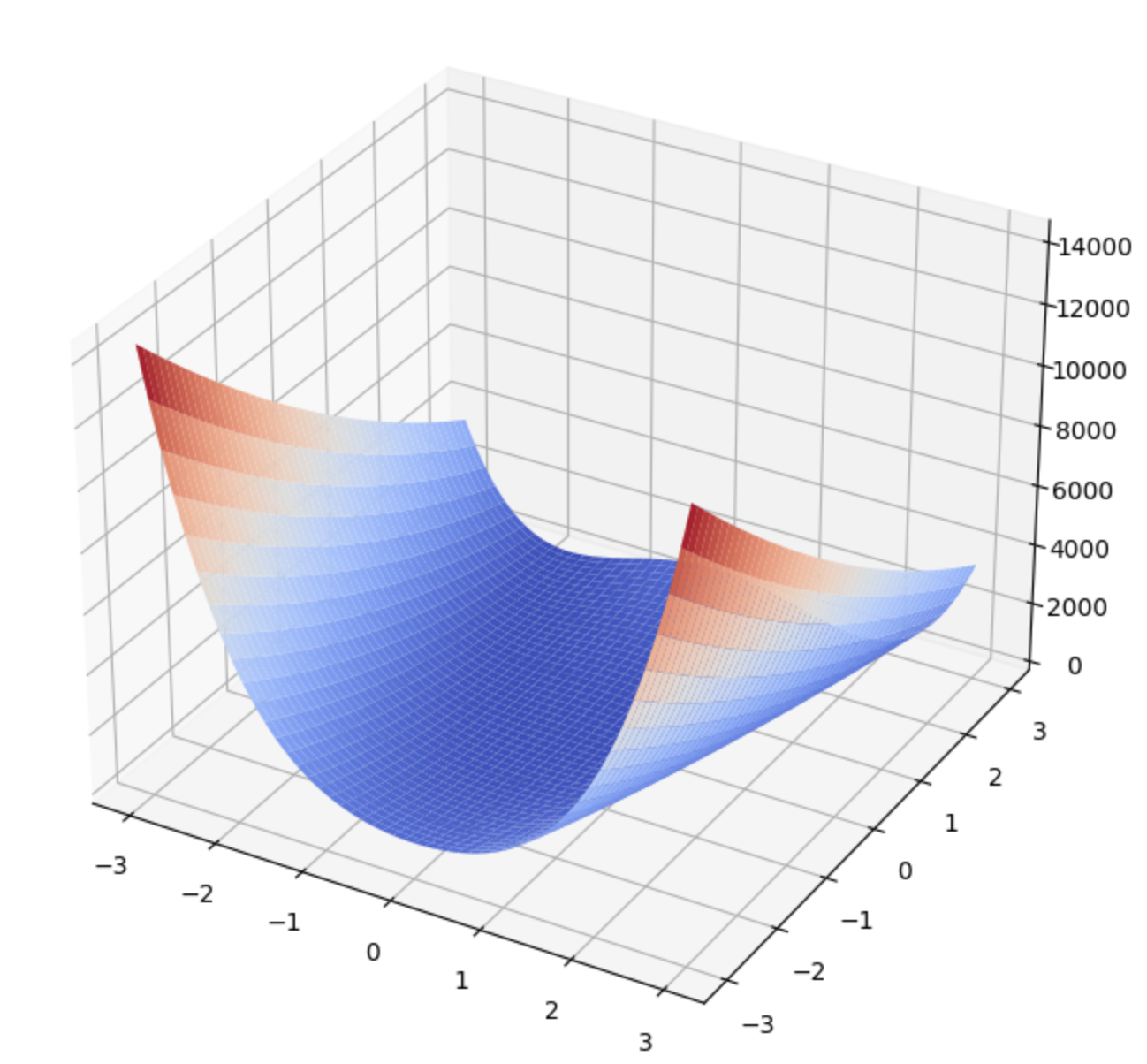
Rosenbrock function

The Rosenbrock function is a widely used test function in optimization and is often used as a performance test for optimization algorithms. Here’s a simple code to plot the Rosenbrock function in Python using Matplotlib:

import numpy as np
import matplotlib.pyplot as plt

def rosenbrock(x, y):
    return (1-x)**2 + 100*(y-x**2)**2

x = np.linspace(-2, 2, 400)
y = np.linspace(-1, 3, 400)
X, Y = np.meshgrid(x, y)
Z = rosenbrock(X, Y)

fig = plt.figure(figsize=(10, 8))
ax = fig.add_subplot(111, projection='3d')
ax.plot_surface(X, Y, Z, cmap='viridis')
ax.set_xlabel('X axis')
ax.set_ylabel('Y axis')
ax.set_zlabel('Z axis')
plt.show()

LP model for Electricity Markets

• Decision variables
  • Generator output: $p_i$ for each generator $i \in G$
  • Power flow: $f_{ij}$ on each edge $(i,j) \in E$
  • Nodal potential $\theta_i$ on each node $i \in N$
• Objective function:
  • minimize the cost of production, $\sum_{i=1}^{G} c_ip_i$
• Constraints:
  • Flow conservation (input=output)
    • for source node $p$ we have: (“sum of everything going out”) - (“sum of everything going in”) = $p$
    • for demand node $d$ we have: (“sum of everything going out”) - (“sum of everything going in” ) = $-d$
    • for node which is neither source nor demand we have: (“sum of everything going out”) - (“sum of everything going in”) = $0$
  • Nodal potential
  • Flow limit constraint
  • Generator physical limit constraint

Inventory Control Problem

• a company must commit to specific production quantity x before knowing the exact demand $d$
• after seeing the demand, the company decides how many to sell and how many to sell at a discounted price of $v$
• This is an example of Decision Making under Uncertainty
• Here and Now decision: production quantity $x$
• Wait and See decision: sell quantity $y$, discount quantity $z$
• Objective: minimize production cost and expected future cost
• Stochastic program:
• $min_{x} cx + E_d[Q(x,d)]$ s.t $0<=x<=\hat{x}$
• $Q(x,d) = min_{y,z} -r.y-s.z$ s.t $y<=d, y+z<=x, y>=0, z>=0$

Generation Capacity Expansion

• An electric utility company plans to build new generation stations to serve growing demand, called generation capacity expansion.
• New generation capacity has to be decided before demand and future fuel price are known
• Future demand and fuel prices are not known at the moment of making capacity decision, but can be estimated as random variables.
• After demand is realized, the utility company schedules existing and new generators based on capacity expansion decision.

Financial Planning

• A family wishes to provide for a child’s college education 12 years later.
• The family currently has 100k and decides how to invest in any of 5 investments
• Investment can be adjusted every 4 years. So there are 3 periods
• The returns of investments are unknown and modeled as random variables
• The family wants to maximize the total expected return
• A problem of decision making under uncertainty

Decision Types

• Here-and-Now: decision made before knowing uncertain parameters
• Wait-and-See: decision made after knowing uncertain parameters

Basic Geometric Objects

Points and vectors

• Point: geometric object in space
• Algebraically, a point in n-dimensional space is given by its coordinates: $x = (x_1, …, x_n)^T \in R^n$
• We always write a vector as a column vector
• A point is also called a vector

Rays, lines, and their parametric forms

• A ray consists of a starting point $a$ and all the points in a direction $d$
• Algebraically it is a set: {$x$ $\in R^n | x = a + \theta d$, $\forall$ $\theta >=0 $}
• A line consists of two rays starting at a point pointing two opposite directions.
• Algebraically it is a set: {$x$ $\in R^n | x = a + \theta d$, $\forall$ $\theta \isin R $}
• For ray and line, it is parametric because a and d are known, and $\theta$ is the parameter

Plane and solutions of linear equations

• A plane in $R^2$ is just a line. $a_1x_1+a_2x_2=c$
• This plane is a line but it is not a parametric representation of a line.
• A plane in $R^3$ is $a_1x_1+a_2x_2+a_3x_3=c$
• If c is 0, plane passes through the origin.

Hyperplane and a Linear equation

• The concept of plane can be extended to any dimension R^n
• Algebraically, $a_1x_1+a_2x_2+…+a_nx_n=c$
• can be written as $a^Tx=c$

Halfspace and a linear inequality

• In $R^2$, a halfspace is half of the whole space
• A halfspace also consists of the line dividing the space
• There are two halfspace in $R^2$, but both include the dividing line
• Same definition can be extended to a halfspace
• $H_1$ = {$x \in R^n: a^Tx>=c$}
• $H_2$ = {$x \in R^n: a^Tx<=c$}

Polyhedron and serveral hyperspaces

• A polyhedron is the intersection of a finite number of halfspaces

Geometric Aspects of Linear Optimization

Corner Points

• Instead of edges, look at Corner Points
• Corner points are responsible for generating the set
• Convex combination of two points in the action of generating it

Convex Combination of Two Points

• Given two points, $a$, $b$ $\in R^n$, a convex combination of $a, b$ is given by
  • $x = \lambda a + (1- \lambda)b$ for some $\lambda \in [0, 1]$
  • Geometrically, x is on the line segment connecting a and b
• Given a point $x$ is a convex combination of $a_1, … a_m$ if $x$ can be written as
  • $x = \sum_{i=1}^m \lambda_ia_i$
  • And, $\sum_{i=1}^m \lambda_i = 1, \lambda_i>=0$ for $i = 1, … , m$
• Corner points are special points, and therefore we give them a special name: Extreme Point
• A point x in a polyhedron P is an extreme point if and only if x is not a convex combination of other two different points in P.

Convex Hull

• A convex hull of $m$ points $a_1, …., a_m$ is the set of all convex combinations of $a_1, .., a_m$ denoted as $conv$ $x{a_1,.., a_n}$
• Theorem: A nonempty and bounded polyhedron is the convex hull of its extreme points.
• A bounded polyhedron is a polyhedron that does not extend to infinity in any direction.

Conic Hull

• A polyhedron is unbounded iff there are directions to move to infinity without leaving the polyhedron.
• Recession direction: a ray that we never leave in the direction of the polyhedron
• However, there are special rays on the edge which can be used to generate all other rays
• A ray $d$ is a conic combination of two rays, $e_1$, $e_2$ if d is a nonnegative weighted sum of $e_1$, $e_2$
• The set of all conic combination of rays $r_1, …, r_m$ is called the conic hull of $r_1, …, r_m$
• The sum of $\lambda$ does not have to equal to 1 here.
• A ray $e$ in a cone C is called an extreme ray, if $e$ is a conic combination of other two different rays in the cone C

Extreme Ray and Extreme Point

• If a polyhedron is bounded, there is no extreme ray
• If a polyhedron is bounded, there must be an extreme point
• If a polyhedron is unbounded, it must have an extreme point

Polyhedron Representations

• Halfspace representation
• Extreme Point representation

Weyl-Caratheodory Theorem

• Any point $x$ in a polyhedron can be written as a sum of two vectors $x = x^’ + d$ where $x^’$ is in the convex hull of its extreme points and d is in the conic hull of its extreme rays.
• $P =$ $conv$ ${x_1, …, x^m} + $ $conic$ ${e^1, …, e^k}$

Algebraic Aspect of Linear Optimization

• Active constraints: A linear constraint that is satisfied as equality at a given point is said to be active or binding at that point. Otherwise, if an inequality constraint is satisfied as strict inequality at a point, it is called inactive.
• Linear independent constraints: If the normal directions of two or more linear constraints are linearly independent, then these constraints are called linearly independent
• Linearly independent active constraints: Active constraints that are linearly independent
• Basic solution: The unique solution of $n$ linearly independent active constraints in $R^n$
• Basic feasible solution (BFS): Basic solution that is feasible.
• Basic Feasible Solution = Extreme Point

Standard Form of writing an LP

• A standard form linear program is written as $min$ $ c^Tx$ $s.t.$ $Ax=b, x>=0 \in X $
• $x \in R^n$ that is, there are $n$ variables
• $A \in R^{m*n}$, ie there are m equality constraints
• We always assume all the $m$ equality constraints are linearly independent
• Equality constraints and Nonnegative constraints on all variables
• The first constraint is data dependent, whereas the second one is not
• Any linear program can be transformed into LP
• Advantage of standard form LP:
  • Complicating constraints are all equality
  • Only inequality constraints are simple, no negativity constraints, which do not depend on data

Basic Solution to standard form LP

• A basic solution is the unique solution to $n$ linearly independent active constraints.
• For a standard form LP, we already have $m$ linearly independent active constraints.
• Need $n-m$ additional linearly independent active constraints
• Where to find them?
• Only from nonnegative constraints: $x_i >= 0$
• But which to choose to make active?
• Choose $m$ such linearly independent columns, denote the corresponding $m*m$ matrix as B, called basis matrix. The corresponding $(n-m)$ $x_i$s are denoted as $x_N$, non basic variables
• Choose $x_i=0$ for all $i$ corresponds to the columns in $N$, $x_N$ = 0

Why do we care?

• Not every LP has a BFS, not every polyhedron has an extreme point (Think about a line or a halfspace)
• So which LP has a BFS?
  • A polyhedron P has an extreme point iff it does not contain a line
  • Corollary: A feasible standard form LP always has a BFS
• If an LP has a finite optimal solution, then an optimal solution is a BFS
• That does not mean all optimal solution must be BFS
• Because feasible standard form LP must have a BFS
• And because an optimal solution must be a BFS
• Then, an optimal solution of standard for LP must be a BFS
• So we only need to look at BFSs, and select the one BFS with the minimum obj cost
• This is why BFS is very important for linear programming.

Local Search

• In a feasible region
• General idea (does not have to be a LP)
• Start from some solution, and move to certain direction to a new point, but stay in feasible region.
• Algorithm

• Generic algorithmic idea
• Gradient Descent and Newton Method uses local search
• Step size should be chosen properly, and the position should be feasible
• Local Search works well for convex optimization (A local minimum of a convex program is also a global minimum)
• Not in general for non convex optimization problems (Local search can get stuck)

Local Search for LP

• We only need to look at basic feasible solution.

• The key step is to find a direction $d$ and step size $\theta$ so that:

  • $d$ points from a BFS to one of its adjacent BFS
  • That adjacent BFS should reduce objective value
  • Move along the favorable direction as much as possible to maintain feasibility and to reduce objective
  • Stop when optimal solution is fount (or cannot be found)

• Two BFS are adjacent if they share the same $n-1$ linearly independent active constraints.

• Two adjacent BFSs must share the same set of $n-m-1$ nonbasic variables as n-m-1 active constraints, and differ in one nonbasic variable.

• Example, if $x=(x_1, …, x_5)$ has nonbasic variables $x_3 = x_4 = x_5 = 0 $, then its adjacent BFS must share two of these three nonbasic variables, i.e. $x_3=x_4=x_2=0$ may be nonbasic variable in an adjacent BFS.

Simplex Method

• The simplex method is a linear programming algorithm that is used to solve optimization problems with linear constraints and a linear objective function. It involves iteratively constructing a sequence of feasible solutions that converge to an optimal solution.
• At each iteration, the simplex method selects a non-basic variable to become basic and then computes a feasible solution by solving a set of linear equations. If the solution is not optimal, the method determines a new non-basic variable to become basic and repeats the process until an optimal solution is found.
• The method is based on the fact that a linear programming problem can be represented graphically as a polyhedron in high-dimensional space, and the optimal solution lies at one of the extreme points of the polyhedron. The simplex method works by traversing the edges of the polyhedron until the optimal extreme point is reached.
• The simplex method is a powerful tool for solving large-scale linear programming problems and is widely used in industry, finance, and other fields. However, it has some limitations, such as its inability to handle nonlinear constraints and its susceptibility to numerical instability when dealing with ill-conditioned matrices.

Degeneracy

• Degeneracy in the simplex method refers to a situation where the simplex algorithm encounters multiple optimal solutions or cycles in the iteration process. In other words, a degenerate linear programming problem has more than one basic feasible solution with the same objective function value.
• Degeneracy can occur when one or more constraints in the linear programming problem are redundant or when there is a linear dependence among the constraints. This leads to a reduced dimensionality in the space of feasible solutions, resulting in more than one optimal solution or cycle in the iteration process.
• Degeneracy can pose challenges for the simplex method since it can lead to slow convergence, cycling, or termination of the algorithm before finding an optimal solution. This is because the simplex method relies on selecting non-basic variables to become basic and constructing a feasible solution by solving a set of linear equations. In a degenerate case, some of the variables may become redundant, leading to cycles in the iteration process.
• To address degeneracy, various modifications to the simplex method have been proposed, such as the use of anti-cycling rules, perturbation techniques, or alternative algorithms such as interior-point methods. These modifications aim to reduce or eliminate the effects of degeneracy on the convergence of the algorithm and ensure finding an optimal solution.

Bland’s rule for degeneracy

• Bland’s rule ensures that the simplex method always chooses the variable with the smallest index as the entering variable and the variable with the smallest subscript as the leaving variable. In other words, Bland’s rule breaks ties in the selection of entering and leaving variables in favor of the variable with the smallest index or subscript.
• By always selecting the variable with the smallest index or subscript, Bland’s rule guarantees that the simplex method cycles through all basic feasible solutions before returning to a previous solution. This eliminates the possibility of the algorithm getting stuck in a cycle and ensures that it converges to an optimal solution eventually.
• Although Bland’s rule can increase the number of iterations required to solve a degenerate linear programming problem, it provides a provably optimal solution and eliminates the possibility of cycling or termination before finding an optimal solution. Bland’s rule is widely used in software implementations of the simplex method and has been shown to be effective in practice.

---

Linear Program Duality

• LP duality is at the core of linear programming theory.
• Provides new perspective on understanding LP, is important for designing algorithms, and has many applications (pricing, game theory, robust optimization, and many more).
• Linear Program (LP) duality is a powerful concept in optimization theory that establishes a relationship between the primal and dual LP problems. The duality principle provides insights into the structure of optimization problems, helps in understanding the solutions and provides a tool for solving LP problems.
• In LP duality, there are two LP problems, known as the primal problem and the dual problem. The primal problem is the original LP problem that seeks to minimize or maximize a linear objective function subject to a set of linear constraints. The dual problem is constructed from the primal problem, and it seeks to maximize or minimize a function subject to a set of constraints.
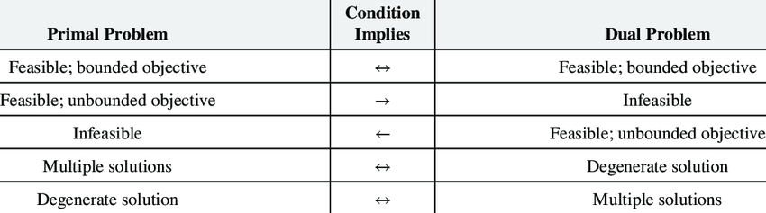
• The duality principle states that the optimal value of the primal problem is equal to the optimal value of the dual problem. Furthermore, the optimal solutions of both problems are related in a specific way. This relationship is known as the duality gap, which is the difference between the optimal values of the primal and dual problems.
• There are two forms of LP duality: weak duality and strong duality. Weak duality states that the optimal value of the dual problem is always greater than or equal to the optimal value of the primal problem. In contrast, strong duality states that if the primal problem has an optimal solution, then the dual problem also has an optimal solution, and the duality gap is zero.
• The dual LP problem provides useful information about the primal LP problem. For example, the dual problem provides a lower bound on the optimal value of the primal problem, and it can be used to derive sensitivity analysis and shadow prices. Additionally, the dual problem can be used to reformulate the primal problem and generate alternative solutions.
• A fundamental motivation of LP duality is to find a systematic way to construct a lower bound to the original LP
• Original LP (Primal LP) $Z_p = min \lbrace c^Tx:Ax=b,x \ge 0 \rbrace $
• Any feasible solution $x$ provides an upper bound on $Z_p$, ie, $Z_p \le c^Tx$
• What about a lower bound, i.e $Z_D \le Z_p$?
• This lower bound is useful because if the lower bound is very close to an upper bound, we have a good estimate of the true optimal.
• However, to get a lower bound, we need to modify the original LP
• In particular, we need to relax the problem.
• Principles of relaxation works for general optimization problems, far beyond LP

Principle of Relaxation

• Relaxation:
  • Find a new objective function that is always smaller or equal to the original objective function at any feasible point
  • Find a feasible region that is larger than the feasible region of the original problem
• Minimize a function lower than the original objective over a region that is larger than the original one. The optimal objective of the new problem will be a lower bound to the original one.
• Among all possible relaxations and lower bounds, find the best lower bound.

Systematic way to carry out relaxation

• Step 1: Relax the objective function
• Step 2: Relax the feasible region by ignoring constraints
  • Separability refers to the property that the objective function of the Lagrangian dual problem can be expressed as the sum of separate functions, each of which depends only on a subset of the variables of the primal problem.
• Step 3 Find the best lower bound.

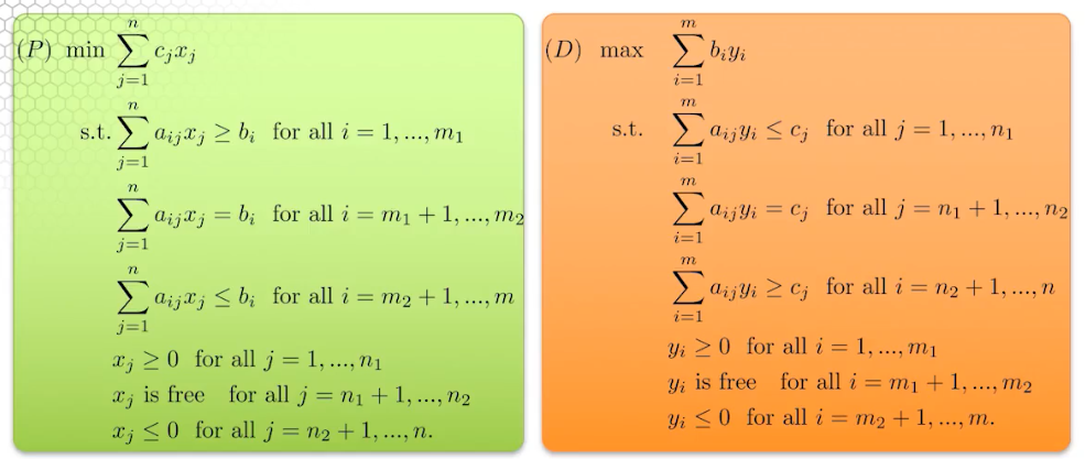
Primal and Dual Pair

Is Lagrangian relaxation a dual problem to the primal?

• Yes, Lagrangian relaxation is a way of obtaining a lower bound on the optimal value of the primal problem by constructing a dual problem.
• In Lagrangian relaxation, the primal problem is first converted into its Lagrangian dual problem by introducing Lagrange multipliers, which are used to form a penalty term that is added to the original objective function. The resulting Lagrangian function is then minimized subject to the constraints, resulting in a lower bound on the optimal value of the primal problem.
• The Lagrangian dual problem is formulated by taking the infimum (minimum) of the Lagrangian over all possible values of the Lagrange multipliers. The dual problem is a maximization problem that seeks to find the maximum value of the infimum, subject to certain constraints that are derived from the original primal problem.
• The duality theorem states that the optimal value of the primal problem is equal to the optimal value of the dual problem, and that any feasible solution to one problem gives a lower bound or upper bound for the other problem. Therefore, Lagrangian relaxation can be seen as a way of constructing the dual problem to the primal problem, and finding a lower bound on the optimal value of the primal problem.

Important

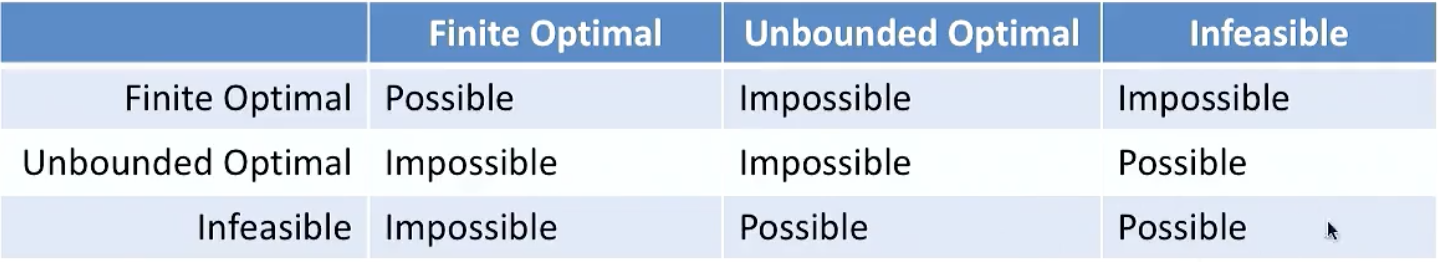
• If a linear program has an unbounded feasible region, then it can either be unbounded or have a finite optimal solution.
• If it has finite optimal solution than its dual must also have finite optimal solution.
• If it is unbounded, then its dual must be infeasible.
• If a linear program has an unbounded feasible region, then its dual problem cannot have an unbounded optimal solution.
• If a linear program has an unbounded feasible region, then its dual may be infeasible or have a finite optimal solution.

Linear Programming weak duality

• Given a primal LP in minimization, by the construction of the dual, the objective value of any feasible solution of the dual problem provides a lower bound to the primal objective cost
• Theorem 1 (Linear programming weak duality): If $x$ is any feasible solution to the primal minimization LP, and y is any feasible solution to the dual maximization LP, then $c^Tx \ge b^Ty$
• This implies:
  • If the optimal cost of the primal minimization problem is $-\inf$ then the dual maximization problem must be infeasible.
  • If the optimal cost of the dual maximization problem is $+\inf$ then the primal minimization problem must be infeasible.
  • Let $x^*$ be feasible to the primal problem and $y*$ be feasible to the dual problem, and suppose $c^Tx^*=b^Ty^*$, then $x^*$ and $y^*$ are optimal solutions to the primal and dual problems, respectively.
• Weak duality does not hold if problem is infeasible.

Strong Duality

• Theorem 1 (Linear programming strong duality): If a primal linear program has a finite optimal solution $x^*$, then its dual linear program must also have a finite optimal solution $y^*$, and the respective optimal objective values are equal, ie, $c^Tx = b^Ty$
• Strong duality is the single most important theorem in LP. Its proof is very illuminating.

Tables of possibilities

SOB method for creating dual of a LP

Complementarity Slackness

• Complementarity slackness is a fundamental concept in optimization theory that arises in the context of solving optimization problems with inequality constraints. It provides insights into the structure of the solutions and helps in understanding the behavior of the constraints in the optimization process.
• In an optimization problem with inequality constraints, the optimal solution typically satisfies the constraints with equality or with some slackness. Complementarity slackness is the condition that ensures that a constraint is either binding (i.e., satisfied with equality) or non-binding (i.e., satisfied with strict inequality) in the optimal solution.
• More formally, let x be a feasible solution to an optimization problem with inequality constraints, and let s be the slack variables associated with the constraints. The complementarity slackness condition requires that the product of the slack variables and the dual variables associated with the constraints is equal to zero.

Robust Optimization

• Making decision during uncertainty
• Robust optimization is a mathematical optimization technique that seeks to find a solution that is optimal under a set of possible scenarios, often in the presence of uncertain or varying parameters. It is particularly useful when dealing with systems that are subject to variability, such as financial or transportation systems, where decisions need to be made under uncertain conditions.
• In robust optimization, instead of trying to find a single optimal solution, a set of feasible solutions is identified that can perform well across a range of possible scenarios. The objective function is typically defined as a worst-case scenario, which ensures that the selected solution is optimal under all possible scenarios.
• Robust optimization can be used in a variety of applications, including portfolio optimization, supply chain management, and resource allocation. It has become increasingly popular in recent years due to its ability to provide robust solutions that can withstand unpredictable changes in the environment.
• We need to formulate constraint in such a way that solution we obtain will allow production to survive all possible realizations of the coefficients.

Large Scale Optimization

Cutting Stock Problem

• The cutting stock problem is a combinatorial optimization problem that involves cutting large sheets of material, such as paper or metal, into smaller pieces of specific sizes in order to minimize waste. The objective is to determine the most efficient cutting pattern that can be used to produce a given number of smaller pieces of the desired sizes, while minimizing the amount of leftover material.
• The cutting stock problem is a common problem in the manufacturing industry, where it is used to optimize the use of raw materials and minimize production costs. It can be formulated as a linear programming problem, where the decision variables are the number of cuts made in each direction, and the objective function is to minimize the amount of leftover material.

Gilmore-Gomory Formulation

• $min \sum_{i=1}^N x_i$, s.t $Ax=b, x \gt 0$
• the coefficients are 1
• where the columns of A are the patterns to cut one large roll
• $b$ is the amount of demand of each size of smaller rolls
• The number of ways to cut a large roll into smaller ones is usually astronomical
• very large number of variables

Column Generation

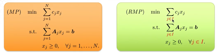
• Pick a subset
• Solve the restricted master problem (RMP)
• A feasible solution of RMP can be made into a feasible solution of MP. This is because RMP has all the constraints in MP.
• A basic feasible solution of RMP can made into a basic feasible solution of MP
• For an optimal BFS of RMP we can compute reduced cost of all nonbasis variables, if any reduced cost is negative, then we know the optimal solution of RMP if not optimal for MP
• We can add the new variable with negative reduced cost to RMP solve the new RMP and repeat the process.
• The procedure of finding a variable with negative reduced cost is called the Pricing Problem. Pricing Problem: Compute all the reduced costs of $x$. If all reduced costs are nonnegative, then $x$ is optimal for MP. Otherwise, we find a new column to add to RMP.

Important

• The features of the cutting stock problem that make column generation a feasible approach to solve:
  • The cutting stock problem formulation has objective coefficients all equal to 1.
  • The cutting stock problem has columns with special structures which can be generated by another optimization problem that is easy to solve.
  • The cutting stock problem has a small number of rows
• The column generation algorithm will terminate if all columns have been added or if no column can further reduce the number of big rolls used to satisfy demand.
• Constraint generation can be used when problems have too many constraints, but not many variables, or with too many rows and not many columns.
• The constraint generation algorithm will terminate if all the constraints are satisfied by the current solution, or if all the contraints are added.

Correctness and Convergence

• The algorithm is correct because of the key properties of RMP
• Does the algorithm converge?
  • Yes, because the algorithm always adds new columns and never disregards any.
  • The worst case is all the columns of MP are used.

Dantzig-Wolfe

• The Dantzig-Wolfe decomposition (also known as the column generation method) is a technique for solving large-scale linear programming problems that have a special structure. It is named after George Dantzig and Philip Wolfe, who first proposed the method in the 1960s.
• The Dantzig-Wolfe decomposition method decomposes a large linear programming problem into smaller sub-problems, each of which can be solved independently. The method is particularly useful when the original problem has a large number of constraints, but only a small number of variables are involved in each constraint.
• The basic idea of the method is to introduce new variables (known as columns) into the problem gradually, one at a time, and to solve the resulting sub-problem using standard linear programming techniques. The optimal solution to the sub-problem is then used to generate a new column, which is added to the problem and the process is repeated until the optimal solution to the original problem is found.
• The Dantzig-Wolfe decomposition method can be used to solve a wide range of linear programming problems, including those with integer variables and those with non-linear objective functions. It is particularly useful for problems that involve complex constraints or require the solution of large-scale optimization problems.

Important

• To use Dantzig-Wolfe decomposition algorithm, the problem must have a special structure where:
  • all constraints are linear and have a block angular structure
  • the objective funciton is a linear function
• We solve Dantzig-Wolfe decomposition by using column generation because:
  • the number of extreme points can be huge
  • there are not many constraints
• The pricing problem is relatively easy to solve because:
  • We can use simplex method instead of enumeration over all the extreme points
  • There are no complicating constraint so that we can solve those pricing problems with angular structures in a distributed manner.

Moore Penrose Pseudoinverse

• The Moore-Penrose pseudoinverse, also known as the Moore-Penrose inverse or simply the pseudoinverse, is a generalization of the matrix inverse for non-square matrices. It is named after Elisha L. Moore and Roger Penrose, who independently introduced the concept in the mid-20th century.
• The pseudoinverse is defined for any m-by-n matrix A, where m and n need not be equal, and it is denoted by A+. The pseudoinverse has several important properties, including:
  • A+AA+A=A+
  • AA+A=AA+
  • (AA+)’=AA+
  • (A+A)A=A
• where A’ denotes the transpose of A.
• The pseudoinverse is useful in a variety of applications, including linear regression, least-squares approximation, and control theory. In particular, if A has linearly independent columns, then A+A is the unique solution to the linear system Ax=b that minimizes the Euclidean norm of the error vector Ax-b.
• The pseudoinverse can be computed using singular value decomposition (SVD) or the QR decomposition. In particular, if A has full column rank, then its pseudoinverse can be computed as A+(A’A)^(-1) where A’ denotes the transpose of A.

Convex Conic Optimization

Nonnegative Orthant cone

• The nonnegative orthant cone is a special type of cone in linear algebra and convex analysis. It is defined as the set of all nonnegative vectors in n-dimensional Euclidean space, denoted as R^n_+, where R^+ denotes the set of nonnegative real numbers.
• Generalizations of linear programming to nonlinear programming through convex cones and generalized inequalities
• A set K is called convex cone if K is convex and $ax \in K$ for all $a \ge 0$ whenever $x \in K$
• What is the relation between order and cone?
  • Order is a comparison relationship between two elements $a$ and $b$, usually written as $a \gt b$
  • An order $\succeq_K$ is defined by an underlying convex cone K as
    • $a \succeq_K b$ iff $a-b \in K$
• A standard form LP can be viewed as
  • $min$ ${c^Tx: Ax=b, x \gt_{R_+^n}0}$
• An elegant way to generalize linear programming is to generalize $R_+^n$ to a general convex cone $K$
• Linear Conic Programming: $min$ $c^T x: Ax=b, x \ge_K 0$
• Linear Conic Programming is a type of optimization problem that involves finding the best solution to a linear objective function subject to a set of linear constraints and the requirement that certain variables lie in a cone. A cone is a set of vectors that satisfies certain properties, such as being non-negative or having a fixed norm.
• In Linear Conic Programming, the constraints are expressed in the form of linear equations or inequalities, while the requirement that certain variables lie in a cone is expressed using conic constraints. Common types of cones include the non-negative orthant, the second-order cone, the semi-definite cone, and the exponential cone.
• The goal of Linear Conic Programming is to find a feasible solution that satisfies all the constraints and optimizes the objective function. This type of optimization problem arises in a variety of applications, such as portfolio optimization, transportation planning, and engineering design. Linear Conic Programming is a powerful tool that can be solved efficiently using specialized algorithms, such as interior-point methods.

Second order cone

• $L^3 = \lbrace (x,y,z) : \sqrt{x^2-y^2} \le z \rbrace$ = $\lbrace(x,y,z):||[x;y]||_2 \le z \rbrace$

Integer optimization

• Integer optimization is a type of optimization problem where the decision variables are required to take integer values. This is in contrast to continuous optimization, where the decision variables can take any real value.
• Integer optimization problems arise in a variety of fields, including operations research, computer science, engineering, and economics. Examples of integer optimization problems include finding the optimal assignment of workers to shifts, determining the best routes for vehicles to travel, and selecting the optimal set of investments to make.
• Integer optimization is often more difficult than continuous optimization, because the feasible set of integer solutions is typically discrete and non-convex. This means that traditional optimization techniques, such as gradient descent, cannot be used. Instead, specialized algorithms, such as branch and bound or cutting plane methods, are used to find optimal or near-optimal solutions.
• Integer optimization is also sometimes referred to as mixed-integer optimization, when the problem includes both integer and continuous decision variables.

Binary Optimization Models

• A special and important class of discrete optimization models are those where the discrete variables and required to be binary, that is, they are required to take values of 0 and 1.
• $min$ $f(x)$ $s.t.$ $g_i(x) \le b_i, x \in R^{n-p} \times \lbrace 0,1 \rbrace^p$

Set Packing, Covering and Partitioning

• Set Packing: A set packing is a collection of sets in which no two sets share a common element. In other words, a set packing is a collection of non-overlapping sets. The objective in set packing is to find the largest possible subset of the sets that do not overlap.
• Set Covering: A set covering is a collection of sets that together contain every element in a given universe. In other words, a set covering is a collection of sets that covers all the elements of a universe. The objective in set covering is to find the smallest possible subset of the sets that covers all the elements.
• Set Partitioning: Set partitioning is a way to divide a set into non-empty subsets such that each element belongs to exactly one subset. In other words, set partitioning is a way to divide a set into mutually exclusive and exhaustive subsets. The objective in set partitioning is to find a partition that satisfies some given criteria.

The set packing problem arises when each set element must appear in at most one subset. In this case, the constraints are of the less-than-or-equal form. The set partitioning problem arises when each set element must appear in exactly one subset, and the constraints in this problem are equality constraints.

Store Location Example

• Where should store be located so that it can maximize the number of customers?
• maximize total customers, constrained to among the locations same location cannot attract more than one city
• pupl is the python package that can be used to model this
• Set Packing: Given $m$ elements and a collection of subsets $S_1, …. , S_n \belongs {1,..,m} with associated nonnegative weights $w_1, …, w_n$ pick sets from this collection such that they are disjoint and the sum of the weights is maximized.

Linear Programming Relaxation

• Decision variable is only taking continuous value to generate the relaxation (drop the integer constraints).
• If LP relaxation is infeasible, so it the IP
• If LP relaxation is unbounded, then the IP can either be infeasible or unbounded.
• If LP relaxation has an optimal solution, then the IP could be infeasible or have an optimal solution
• It always holds that $v_{LP} \le v_{IP}$
• If an optimal solution to the LP is an integer, then it is an optimal solution to the IP.
• It’s solution can sometimes be rounded to get a good solution to the IP

Ideal Formulations

• Stronger Formulation: Stronger formulation lead to stronger LP relaxations, and so better LP relaxation better bounds, and sometimes LP relaxations solutions that are feasible to the MLP
• The formulation of an MLP can be strengthened
  • by adding constraints (valid inequalities)
  • by tightening constraint coefficients
  • by introducing new variables and constraints
• An ideal formulation of a MILP is one whose LP relaxation solves the MLP
• Ideal formulations are hard to obtain, so we strive to obtain strong formulation that approximate the ideal formulation

Branch Bound Algorithm

• Branch and bound is a popular algorithm used for solving mixed-integer linear programming (MILP) problems. The basic idea behind branch and bound is to divide the problem into smaller subproblems, solve each subproblem separately, and then combine the solutions to obtain an overall solution to the original problem.
• Here are the steps involved in the branch and bound algorithm for MILP:
  • Solve the relaxed linear programming (LP) problem, which is the MILP problem with the integer constraints removed. This provides an initial solution to the MILP problem.
  • If the LP solution satisfies all the integer constraints, then we have found an optimal solution to the MILP problem. Otherwise, select one of the integer variables with a non-integer value in the LP solution.
  • Create two new subproblems by branching on the selected variable: one subproblem where the variable is fixed to its integer floor, and another subproblem where the variable is fixed to its integer ceiling.
  • Solve each of the subproblems using the LP solver. If a subproblem has an integer solution that is worse than the current best solution, we can prune that branch of the search tree. Otherwise, continue branching until we have found an optimal integer solution or all branches have been pruned.
  • Once all branches have been pruned, the best integer solution found during the search is the optimal solution to the MILP problem.